


Dolph-Chebyshev Window Theory
In this section, the main elements of the theory behind the Dolph-Chebyshev window are summarized.
Chebyshev Polynomials
![\includegraphics[width=\twidth]{eps/first-even-chebs-c}](http://www.dsprelated.com/josimages_new/sasp2/img533.png)
The ![]() th Chebyshev polynomial may be defined by
th Chebyshev polynomial may be defined by
![$\displaystyle T_n(x) = \left\{\begin{array}{ll} \cos[n\cos^{-1}(x)], & \vert x\vert\le1 \\ [5pt] \cosh[n\cosh^{-1}(x)], & \vert x\vert>1 \\ \end{array} \right..$](http://www.dsprelated.com/josimages_new/sasp2/img534.png) |
(4.46) |
The first three even-order cases are plotted in Fig.3.35. (We will only need the even orders for making Chebyshev windows, as only they are symmetric about time 0.) Clearly,
| (4.47) |
for
 is an
is an  th-order polynomial in
  .
.
-
is an even function when
is an even integer,
and odd when
is odd.
-
has
zeros in the open interval
 , and
, and
 extrema in the closed interval
 ![$ [-1,1]$](http://www.dsprelated.com/josimages_new/sasp2/img543.png) .
.
 for
for  .
.
Dolph-Chebyshev Window Definition
Let ![]() denote the desired window length. Then the zero-phase
Dolph-Chebyshev window is defined in the frequency domain by
[155]
denote the desired window length. Then the zero-phase
Dolph-Chebyshev window is defined in the frequency domain by
[155]
![$\displaystyle W(\omega) = \frac{T_{M-1}[x_0 \cos(\omega/2)]}{T_{M-1}(x_0)}$](http://www.dsprelated.com/josimages_new/sasp2/img546.png) |
(4.48) |
where
 |
(4.49) |
where
![$\displaystyle \omega_c \isdefs 2\cos^{-1}\left[\frac{1}{x_0}\right].$](http://www.dsprelated.com/josimages_new/sasp2/img549.png) |
(4.50) |
Expanding
 |
(4.51) |
where
 . Thus, the coefficients
Dolph-Chebyshev Window Main-Lobe Width
Given the window length ![]() and ripple magnitude
and ripple magnitude ![]() , the main-lobe
width
, the main-lobe
width ![]() may be computed as follows [155]:
may be computed as follows [155]:
![\begin{eqnarray*}
x_0 &=& \cosh\left[\frac{\cosh^{-1}\left(\frac{1}{r}\right)}{M-1}\right]\\
\omega_c &=& 2\cos^{-1}\left(\frac{1}{x_0}\right)
\end{eqnarray*}](http://www.dsprelated.com/josimages_new/sasp2/img553.png)
This is the smallest main-lobe width possible for the given window length and side-lobe spec.
Dolph-Chebyshev Window Length Computation
Given a prescribed side-lobe ripple-magnitude ![]() and main-lobe width
and main-lobe width
![]() , the required window length
, the required window length ![]() is given by [155]
is given by [155]
![$\displaystyle M = 1 + \frac{\cosh^{-1}(1/r)}{\cosh^{-1}[\sec(\omega_c/2)]}.$](http://www.dsprelated.com/josimages_new/sasp2/img554.png) |
(4.52) |
For
 |
(4.53) |
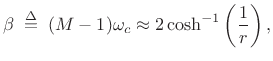
Thus, half the time-bandwidth product in radians is approximately
 |
(4.54) |
where
Next Section:
Matlab for the Gaussian Window
Previous Section:
Chebyshev and Hamming Windows Compared


