


Optimal (but poor if unweighted)
Least-Squares
Impulse Response Design
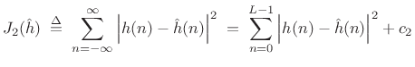
Perhaps the most commonly employed error criterion in signal processing is the least-squares error criterion.
Let ![]() denote some ideal filter impulse response, possibly
infinitely long, and let
denote some ideal filter impulse response, possibly
infinitely long, and let
![]() denote the impulse response of a
length
denote the impulse response of a
length ![]() causal FIR filter that we wish to design. The sum of
squared errors is given by
causal FIR filter that we wish to design. The sum of
squared errors is given by
 |
(5.4) |
where
![$\displaystyle {\hat h}(n) \isdef \left\{\begin{array}{ll} h(n), & 0\leq n \leq L-1 \\ [5pt] 0, & \hbox{otherwise} \\ \end{array} \right. \protect$](http://www.dsprelated.com/josimages_new/sasp2/img681.png)
The same solution works also for any
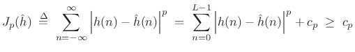 |
(5.6) |
is also minimized by matching the leading
In the ![]() (least-squares) case, we have, by the Fourier energy
theorem (§2.3.8),
(least-squares) case, we have, by the Fourier energy
theorem (§2.3.8),
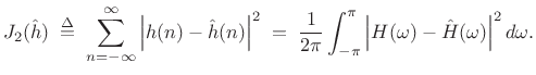 |
(5.7) |
Therefore,
Examples
Figure 4.3 shows the amplitude response of a length ![]() optimal least-squares FIR lowpass filter, for the case in which the
cut-off frequency is one-fourth the sampling rate (
optimal least-squares FIR lowpass filter, for the case in which the
cut-off frequency is one-fourth the sampling rate (![]() ).
).
![\includegraphics[width=\twidth]{eps/ilpftdlsL30}](http://www.dsprelated.com/josimages_new/sasp2/img688.png) |
We see that, although the impulse response is optimal in the
least-squares sense (in fact optimal under any ![]() norm with any
error-weighting), the filter is quite poor from an audio
perspective. In particular, the stop-band gain, in which zero is
desired, is only about 10 dB down. Furthermore, increasing the length
of the filter does not help, as evidenced by the length 71 result in
Fig.4.4.
norm with any
error-weighting), the filter is quite poor from an audio
perspective. In particular, the stop-band gain, in which zero is
desired, is only about 10 dB down. Furthermore, increasing the length
of the filter does not help, as evidenced by the length 71 result in
Fig.4.4.
![\includegraphics[width=\twidth]{eps/ilpftdlsL71}](http://www.dsprelated.com/josimages_new/sasp2/img689.png) |
It is not the case that a length ![]() FIR filter is too short for
implementing a reasonable audio lowpass filter, as can be seen in
Fig.4.5. The optimal Chebyshev lowpass filter in
this figure was designed by the Matlab statement
FIR filter is too short for
implementing a reasonable audio lowpass filter, as can be seen in
Fig.4.5. The optimal Chebyshev lowpass filter in
this figure was designed by the Matlab statement
hh = firpm(L-1,[0 0.5 0.6 1],[1 1 0 0]);where, in terms of the lowpass design specs defined in §4.2 above, we are asking for
-
 (pass-band edge frequency)5.5
-
 (stop-band edge frequency)
![\includegraphics[width=\twidth]{eps/ilpfchebL71}](http://www.dsprelated.com/josimages_new/sasp2/img696.png) |
We see that the Chebyshev design has a stop-band attenuation better than 60 dB, no corner-frequency resonance, and the error is equiripple in both stop-band (visible) and pass-band (not visible). Note also that there is a transition band between the pass-band and stop-band (specified in the call to firpm as being between normalized frequencies 0.5 and 0.6).
The main problem with the least-squares design examples above is the
absence of a transition band specification. That is, the
filter specification calls for an infinite roll-off rate from the
pass-band to the stop-band, and this cannot be accomplished by any FIR
filter. (Review Fig.4.2 for an illustration of more
practical lowpass-filter design specifications.) With a transition
band and a weighting function, least-squares FIR filter design can
perform very well in practice. As a rule of thumb, the transition
bandwidth should be at least ![]() , where
, where ![]() is the FIR filter
length in samples. (Recall that the main-lobe width of a length
is the FIR filter
length in samples. (Recall that the main-lobe width of a length ![]() rectangular window is
rectangular window is ![]() (§3.1.2).) Such a rule
respects the basic Fourier duality of length in the time domain and
``minimum feature width'' in the frequency domain.
(§3.1.2).) Such a rule
respects the basic Fourier duality of length in the time domain and
``minimum feature width'' in the frequency domain.
Next Section:
Frequency Sampling Method for FIR Filter Design
Previous Section:
Lowpass Filter Design Specifications


