


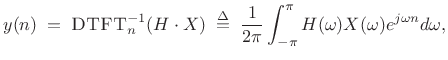
FIR Digital Filter Design
FIR filters are basic in spectral audio signal processing. In fact,
the fastest way to implement long FIR filters in conventional
CPUs5.1 is by means of
FFT convolution.
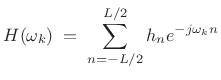
The
convolution theorem for Fourier transforms (§2.3.5)
states that the convolution of an input signal ![]() with a filter
impulse-response
with a filter
impulse-response ![]() is given by the inverse DTFT of the product of
the signal's spectrum
is given by the inverse DTFT of the product of
the signal's spectrum ![]() times the filter's frequency
response
times the filter's frequency
response ![]() , i.e.,
, i.e.,
 |
(5.1) |
where
and the DTFT is defined as (§2.1)
 |
(5.2) |
As usual with the DTFT, the sampling rate is assumed to be
This chapter provides a starting point in the area of FIR digital filter design. The so-called ``window method'' for FIR filter design, also based on the convolution theorem for Fourier transforms, is discussed in some detail, and compared with an optimal Chebyshev method. Other methods, such as least-squares, are discussed briefly to provide further perspective. Tools for FIR filter design in both Octave and the Matlab Signal Processing Toolbox are listed where applicable. For more information on digital filter design, see, e.g., the documentation for the Matlab Signal Processing Toolbox and/or [263,283,32,204,275,224,198,258].
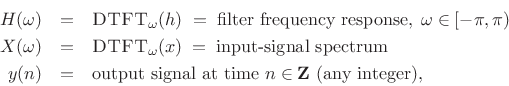
The Ideal Lowpass Filter
Consider the ideal lowpass filter, depicted in Fig.4.1.
An ideal lowpass may be characterized by a gain of 1 for all
frequencies below some cut-off frequency ![]() in Hz, and a
gain of 0 for all higher frequencies.5.2
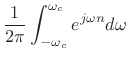
The impulse response of the ideal lowpass filter
is easy to calculate:
in Hz, and a
gain of 0 for all higher frequencies.5.2
The impulse response of the ideal lowpass filter
is easy to calculate:
![$\displaystyle \frac{1}{2\pi}\int_{-\pi}^{\pi} d\omega e^{j\omega n }
\left\{\begin{array}{ll}
1, & \left\vert\omega\right\vert\leq\omega_c \\ [5pt]
0, & \mbox{otherwise} \\
\end{array} \right.$](http://www.dsprelated.com/josimages_new/sasp2/img653.png)
![$\displaystyle \frac{1}{2\pi jn}\left[e^{j\omega_c n} - e^{-j\omega_c n}\right]$](http://www.dsprelated.com/josimages_new/sasp2/img655.png)

where
 denotes the normalized cut-off
frequency in radians per sample. Thus, the impulse response of an
ideal lowpass filter is a sinc function.
denotes the normalized cut-off
frequency in radians per sample. Thus, the impulse response of an
ideal lowpass filter is a sinc function.
Unfortunately, we cannot implement the ideal lowpass filter in
practice because its impulse response is infinitely long in
time. It is also noncausal; it cannot be shifted to make it
causal because the impulse response extends all the way to time
![]() . It is clear we will have to accept some sort of
compromise in the design of any practical lowpass filter.
. It is clear we will have to accept some sort of
compromise in the design of any practical lowpass filter.
The subject of digital filter design is generally concerned with finding an optimal approximation to the desired frequency response by minimizing some norm of a prescribed error criterion with respect to a set of practical filter coefficients, perhaps subject also to some constraints (usually linear equality or inequality constraints) on the filter coefficients, as we saw for optimal window design in §3.13.5.3In audio applications, optimality is difficult to define precisely because perception is involved. It is therefore valuable to consider also suboptimal methods that are ``close enough'' to optimal, and which may have other advantages such as extreme simplicity and/or speed. We will examine some specific cases below.
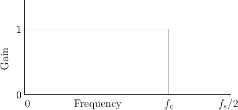
Lowpass Filter Design Specifications
Typical design parameters for a lowpass filter are shown in Fig.4.2.
![\includegraphics[width=4in]{eps/idealFilter}](http://www.dsprelated.com/josimages_new/sasp2/img661.png)
The design parameters are defined as follows:
-
 stop-band ripple (
 dB is common)
-
 pass-band ripple (
 dB typical)
-
 stop-band edge frequency
-
 pass-band edge frequency
- TW: transition width

- SBA: stop-band attenuation
In terms of these specifications, we may define an optimal FIR lowpass filter of a given length to be one which minimizes the stop-band and pass-band ripple (weighted relatively as desired) for given stop-band and pass-band edge frequencies. Such optimal filters are often designed in practice by Chebyshev methods, as we encountered already in the study of windows for spectrum analysis (§3.10,§3.13). Optimal Chebyshev FIR filters will be discussed further below (in §4.5.2), but first we look at simpler FIR design methods and compare to optimal Chebyshev designs for reference. An advantage of the simpler methods is that they are more suitable for interactive, real-time, and/or signal-adaptive FIR filter design.
Ideal Lowpass Filter Revisited
The ideal lowpass filter of Fig.4.1 can now be described by the following specifications:
- The transition width TW is zero (
 in Fig.4.2).
- The pass-band and stop-band ripples are both zero
( in Fig.4.2, and
 ).
).
Optimal (but poor if unweighted)
Least-Squares
Impulse Response Design
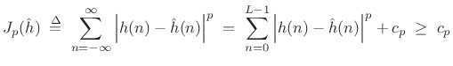
Perhaps the most commonly employed error criterion in signal processing is the least-squares error criterion.
Let ![]() denote some ideal filter impulse response, possibly
infinitely long, and let
denote some ideal filter impulse response, possibly
infinitely long, and let
![]() denote the impulse response of a
length
denote the impulse response of a
length ![]() causal FIR filter that we wish to design. The sum of
squared errors is given by
causal FIR filter that we wish to design. The sum of
squared errors is given by
 |
(5.4) |
where
![$\displaystyle {\hat h}(n) \isdef \left\{\begin{array}{ll} h(n), & 0\leq n \leq L-1 \\ [5pt] 0, & \hbox{otherwise} \\ \end{array} \right. \protect$](http://www.dsprelated.com/josimages_new/sasp2/img681.png)
The same solution works also for any
 |
(5.6) |
is also minimized by matching the leading
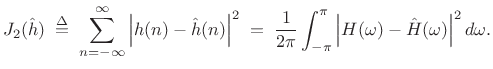
In the ![]() (least-squares) case, we have, by the Fourier energy
theorem (§2.3.8),
(least-squares) case, we have, by the Fourier energy
theorem (§2.3.8),
 |
(5.7) |
Therefore,
Examples
Figure 4.3 shows the amplitude response of a length ![]() optimal least-squares FIR lowpass filter, for the case in which the
cut-off frequency is one-fourth the sampling rate (
optimal least-squares FIR lowpass filter, for the case in which the
cut-off frequency is one-fourth the sampling rate (![]() ).
).
![\includegraphics[width=\twidth]{eps/ilpftdlsL30}](http://www.dsprelated.com/josimages_new/sasp2/img688.png) |
We see that, although the impulse response is optimal in the
least-squares sense (in fact optimal under any ![]() norm with any
error-weighting), the filter is quite poor from an audio
perspective. In particular, the stop-band gain, in which zero is
desired, is only about 10 dB down. Furthermore, increasing the length
of the filter does not help, as evidenced by the length 71 result in
Fig.4.4.
norm with any
error-weighting), the filter is quite poor from an audio
perspective. In particular, the stop-band gain, in which zero is
desired, is only about 10 dB down. Furthermore, increasing the length
of the filter does not help, as evidenced by the length 71 result in
Fig.4.4.
![\includegraphics[width=\twidth]{eps/ilpftdlsL71}](http://www.dsprelated.com/josimages_new/sasp2/img689.png) |
It is not the case that a length ![]() FIR filter is too short for
implementing a reasonable audio lowpass filter, as can be seen in
Fig.4.5. The optimal Chebyshev lowpass filter in
this figure was designed by the Matlab statement
FIR filter is too short for
implementing a reasonable audio lowpass filter, as can be seen in
Fig.4.5. The optimal Chebyshev lowpass filter in
this figure was designed by the Matlab statement
hh = firpm(L-1,[0 0.5 0.6 1],[1 1 0 0]);where, in terms of the lowpass design specs defined in §4.2 above, we are asking for
-
 (pass-band edge frequency)5.5
-
 (stop-band edge frequency)
![\includegraphics[width=\twidth]{eps/ilpfchebL71}](http://www.dsprelated.com/josimages_new/sasp2/img696.png) |
We see that the Chebyshev design has a stop-band attenuation better than 60 dB, no corner-frequency resonance, and the error is equiripple in both stop-band (visible) and pass-band (not visible). Note also that there is a transition band between the pass-band and stop-band (specified in the call to firpm as being between normalized frequencies 0.5 and 0.6).
The main problem with the least-squares design examples above is the
absence of a transition band specification. That is, the
filter specification calls for an infinite roll-off rate from the
pass-band to the stop-band, and this cannot be accomplished by any FIR
filter. (Review Fig.4.2 for an illustration of more
practical lowpass-filter design specifications.) With a transition
band and a weighting function, least-squares FIR filter design can
perform very well in practice. As a rule of thumb, the transition
bandwidth should be at least ![]() , where
, where ![]() is the FIR filter
length in samples. (Recall that the main-lobe width of a length
is the FIR filter
length in samples. (Recall that the main-lobe width of a length ![]() rectangular window is
rectangular window is ![]() (§3.1.2).) Such a rule
respects the basic Fourier duality of length in the time domain and
``minimum feature width'' in the frequency domain.
(§3.1.2).) Such a rule
respects the basic Fourier duality of length in the time domain and
``minimum feature width'' in the frequency domain.
Frequency Sampling Method for
FIR Filter Design
The frequency-sampling method for FIR filter design is perhaps the simplest and most direct technique imaginable when a desired frequency response has been specified. It consists simply of uniformly sampling the desired frequency response, and performing an inverse DFT to obtain the corresponding (finite) impulse response [224, pp. 105-23], [198, pp. 251-55]. The results are not optimal, however, because the response generally deviates from what is desired between the samples. When the desired frequency-response is undersampled, which is typical, the resulting impulse response will be time aliased to some extent. It is important to evaluate the final impulse response via a simulated DTFT (FFT with lots of zero padding), comparing to the originally desired frequency response.
The frequency-sampling method for FIR filter design is illustrated in §4.6.2 below in the context of the window method for FIR filter design, to which we now turn.
Window Method for FIR Filter Design
The window method for digital filter design is fast, convenient, and robust, but generally suboptimal. It is easily understood in terms of the convolution theorem for Fourier transforms, making it instructive to study after the Fourier theorems and windows for spectrum analysis. It can be effectively combined with the frequency sampling method, as we will see in §4.6 below.
The window method consists of simply ``windowing'' a theoretically
ideal filter impulse response ![]() by some suitably chosen window
function
by some suitably chosen window
function ![]() , yielding
, yielding
| (5.8) |
For example, as derived in Eq.
 |
(5.9) |
where
Since
![]() sinc
sinc![]() decays away from time 0 as
decays away from time 0 as ![]() , we would
expect to be able to truncate it to the interval
, we would
expect to be able to truncate it to the interval ![]() , for some
sufficiently large
, for some
sufficiently large ![]() , and obtain a pretty good FIR filter which
approximates the ideal filter. This would be an example of using the
window method with the rectangular window. We saw in
§4.3 that such a choice is optimal in the least-squares
sense, but it designs relatively poor audio filters. Choosing other
windows corresponds to tapering the ideal impulse response to
zero instead of truncating it. Tapering better preserves the shape of
the desired frequency response, as we will see. By choosing the
window carefully, we can manage various trade-offs so as to maximize
the filter-design quality in a given application.
, and obtain a pretty good FIR filter which
approximates the ideal filter. This would be an example of using the
window method with the rectangular window. We saw in
§4.3 that such a choice is optimal in the least-squares
sense, but it designs relatively poor audio filters. Choosing other
windows corresponds to tapering the ideal impulse response to
zero instead of truncating it. Tapering better preserves the shape of
the desired frequency response, as we will see. By choosing the
window carefully, we can manage various trade-offs so as to maximize
the filter-design quality in a given application.
Window functions are always time limited. This means there is
always a finite integer ![]() such that
such that ![]() for all
for all
![]() . The final windowed impulse response
. The final windowed impulse response
![]() is thus always time-limited, as needed for practical
implementation. The window method always designs a
finite-impulse-response (FIR) digital filter (as opposed to an
infinite-impulse-response (IIR) digital filter).
is thus always time-limited, as needed for practical
implementation. The window method always designs a
finite-impulse-response (FIR) digital filter (as opposed to an
infinite-impulse-response (IIR) digital filter).
By the dual of the convolution theorem, pointwise multiplication in
the time domain corresponds to convolution in the frequency domain.
Thus, the designed filter ![]() has a frequency response given by
has a frequency response given by
| (5.10) |
where
- The pass-band gain is primarily the area under the
main lobe of the window transform, provided the main lobe
``fits'' inside the pass-band (i.e., the total lowpass bandwidth
 is greater than or equal to the main-lobe width
of
is greater than or equal to the main-lobe width
of  ).
).
- The stop-band gain is given by an integral over a portion
of the side lobes of the window transform. Since side-lobes
oscillate about zero, a finite integral over them is normally much
smaller than the side-lobes themselves, due to adjacent side-lobe
cancellation under the integral.
- The best stop-band performance occurs when the cut-off
frequency is set so that the stop-band side-lobe integral traverses a
whole number of side lobes.
- The transition bandwidth is equal to the bandwidth of
the main lobe of the window transform, again provided that the main
lobe ``fits'' inside the pass-band.
- For very small lowpass bandwidths
 ,
,  approaches an
impulse in the frequency domain. Since the impulse is the
identity operator under convolution, the resulting lowpass filter
approaches an
impulse in the frequency domain. Since the impulse is the
identity operator under convolution, the resulting lowpass filter
 approaches the window transform
  for small
. In particular, the stop-band gain approaches the window
side-lobe level, and the transition width approaches half the
main-lobe width. Thus, for good results, the lowpass cut-off
frequency should be set no lower than half the window's main-lobe
width.
for small
. In particular, the stop-band gain approaches the window
side-lobe level, and the transition width approaches half the
main-lobe width. Thus, for good results, the lowpass cut-off
frequency should be set no lower than half the window's main-lobe
width.
Matlab Support for the Window Method
Octave and the Matlab Signal Processing Toolbox have two functions implementing the window method for FIR digital filter design:
- fir1 designs lowpass, highpass, bandpass, and
multi-bandpass filters.
- fir2 takes an arbitrary magnitude frequency response
specification.
Bandpass Filter Design Example
The matlab code below designs a bandpass filter which passes
frequencies between 4 kHz and 6 kHz, allowing transition bands from 3-4
kHz and 6-8 kHz (i.e., the stop-bands are 0-3 kHz and 8-10 kHz, when the
sampling rate is 20 kHz). The desired stop-band attenuation is 80 dB,
and the pass-band ripple is required to be no greater than 0.1 dB. For
these specifications, the function kaiserord returns a beta
value of
![]() and a window length of
and a window length of ![]() . These values
are passed to the function kaiser which computes the window
function itself. The ideal bandpass-filter impulse response is
computed in fir1, and the supplied Kaiser window is applied
to shorten it to length
. These values
are passed to the function kaiser which computes the window
function itself. The ideal bandpass-filter impulse response is
computed in fir1, and the supplied Kaiser window is applied
to shorten it to length ![]() .
.
fs = 20000;                 % sampling rate
F = [3000 4000 6000 8000];  % band limits
A = [0 1 0];                % band type: 0='stop', 1='pass'
dev = [0.0001 10^(0.1/20)-1 0.0001]; % ripple/attenuation spec
[M,Wn,beta,typ] = kaiserord(F,A,dev,fs);  % window parameters
b = fir1(M,Wn,typ,kaiser(M+1,beta),'noscale'); % filter design
Note the conciseness of the matlab code thanks to the use of kaiserord and fir1 from Octave or the Matlab Signal Processing Toolbox.
Figure 4.6 shows the magnitude frequency response
![]() of the resulting FIR filter
of the resulting FIR filter ![]() . Note that
the upper pass-band edge has been moved to 6500 Hz instead of 6000 Hz,
and the stop-band begins at 7500 Hz instead of 8000 Hz as requested.
While this may look like a bug at first, it's actually a perfectly
fine solution. As discussed earlier (§4.5), all
transition-widths in filters designed by the window method must equal
the window-transform's main-lobe width. Therefore, the only way to
achieve specs when there are multiple transition regions specified is
to set the main-lobe width to the minimum transition width.
For the others, it makes sense to center the transition within
the requested transition region.
. Note that
the upper pass-band edge has been moved to 6500 Hz instead of 6000 Hz,
and the stop-band begins at 7500 Hz instead of 8000 Hz as requested.
While this may look like a bug at first, it's actually a perfectly
fine solution. As discussed earlier (§4.5), all
transition-widths in filters designed by the window method must equal
the window-transform's main-lobe width. Therefore, the only way to
achieve specs when there are multiple transition regions specified is
to set the main-lobe width to the minimum transition width.
For the others, it makes sense to center the transition within
the requested transition region.
![\includegraphics[width=\twidth]{eps/fltDesign}](http://www.dsprelated.com/josimages_new/sasp2/img724.png)
Under the Hood of kaiserord
Without kaiserord, we would need to implement Kaiser's
formula [115,67] for estimating the Kaiser-window
![]() required to achieve the given filter specs:
required to achieve the given filter specs:
![$\displaystyle \beta = \left\{\begin{array}{ll} 0.1102(A-8.7), & A > 50 \\ [5pt] 0.5842(A-21)^{0.4} + 0.07886(A-21), & 21< A < 50 \\ [5pt] 0, & A < 21, \\ \end{array} \right. \protect$](http://www.dsprelated.com/josimages_new/sasp2/img725.png)
where
A similar function from [198] for window design (as opposed to filter design5.7) is
![$\displaystyle \beta = \left\{\begin{array}{ll} 0, & A<13.26 \\ [5pt] 0.76609(A-13.26)^{0.4} + 0.09834(A-13.26), & 13.26< A < 60 \\ [5pt] 0.12438*(A+6.3), & 60<A<120, \\ \end{array} \right. \protect$](http://www.dsprelated.com/josimages_new/sasp2/img728.png)
where now
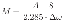
Similarly, the filter order ![]() is estimated from stop-band
attenuation
is estimated from stop-band
attenuation ![]() and desired transition width
and desired transition width
![]() using the
empirical formula
using the
empirical formula
 |
(5.13) |
where
Without the function fir1, we would have to manually
implement the window method of filter design by (1) constructing the
impulse response of the ideal bandpass filter ![]() (a cosine
modulated sinc function), (2) computing the Kaiser window
(a cosine
modulated sinc function), (2) computing the Kaiser window ![]() using
the estimated length and
using
the estimated length and ![]() from above, then finally (3)
windowing the ideal impulse response with the Kaiser window to obtain
the FIR filter coefficients
from above, then finally (3)
windowing the ideal impulse response with the Kaiser window to obtain
the FIR filter coefficients
![]() . A manual design of
this nature will be illustrated in the Hilbert transform example of
§4.6.
. A manual design of
this nature will be illustrated in the Hilbert transform example of
§4.6.
Comparison to the Optimal Chebyshev FIR Bandpass Filter
To provide some perspective on the results, let's compare the window method to the optimal Chebyshev FIR filter (§4.10) for the same length and design specifications above.
The following Matlab code illustrates two different bandpass filter designs. The first (different transition bands) illustrates a problem we'll look at. The second (equal transition bands, commented out), avoids the problem.
M = 101;
normF = [0 0.3 0.4 0.6 0.8 1.0];  % transition bands different
%normF = [0 0.3 0.4 0.6 0.7 1.0]; % transition bands the same
amp = [0 0 1 1 0 0];              % desired amplitude in each band

[b2,err2] = firpm(M-1,normF,amp); % optimal filter of length M
Figure 4.7 shows the frequency response of the Chebyshev FIR filter designed by firpm, to be compared with the window-method FIR filter in Fig.4.6. Note that the upper transition band ``blows up''. This is a well known failure mode in FIR filter design using the Remez exchange algorithm [176,224]. It can be eliminated by narrowing the transition band, as shown in Fig.4.8. There is no error penalty in the transition region, so it is necessary that each one be ``sufficiently narrow'' to avoid this phenomenon.
Remember the rule of thumb that the narrowest transition-band possible
for a length ![]() FIR filter is on the order of
FIR filter is on the order of ![]() , because
that's the width of the main-lobe of a length
, because
that's the width of the main-lobe of a length ![]() rectangular window
(measured between zero-crossings) (§3.1.2). Therefore, this
value is quite exact for the transition-widths of FIR bandpass filters
designed by the window method using the rectangular window (when the
main-lobe fits entirely within the adjacent pass-band and stop-band).
For a Hamming window, the window-method transition width would instead
be
rectangular window
(measured between zero-crossings) (§3.1.2). Therefore, this
value is quite exact for the transition-widths of FIR bandpass filters
designed by the window method using the rectangular window (when the
main-lobe fits entirely within the adjacent pass-band and stop-band).
For a Hamming window, the window-method transition width would instead
be ![]() . Thus, we might expect an optimal Chebyshev design to
provide transition widths in the vicinity of
. Thus, we might expect an optimal Chebyshev design to
provide transition widths in the vicinity of ![]() , but probably
not too close to
, but probably
not too close to ![]() or below
In the example above, where the sampling rate was
or below
In the example above, where the sampling rate was ![]() kHz, and the
filter length was
kHz, and the
filter length was ![]() , we expect to be able to achieve transition
bands circa
, we expect to be able to achieve transition
bands circa
![]() Hz, but not so low
as
Hz, but not so low
as
![]() Hz. As we found above,
Hz. As we found above,
![]() Hz was under-constrained, while
Hz was under-constrained, while ![]() Hz was ok, being near
the ``Hamming transition width.''
Hz was ok, being near
the ``Hamming transition width.''
![\includegraphics[width=\twidth]{eps/fltDesignRemez}](http://www.dsprelated.com/josimages_new/sasp2/img738.png) |
![\includegraphics[width=\twidth]{eps/fltDesignRemezTighter}](http://www.dsprelated.com/josimages_new/sasp2/img739.png) |
Hilbert Transform Design Example
We will now use the window method to design a complex bandpass filter which passes positive frequencies and rejects negative frequencies.
Since every real signal ![]() possesses a Hermitian spectrum
possesses a Hermitian spectrum
![]() , i.e.,
, i.e.,
![]() , it follows that, if
we filter out the negative frequencies, we will destroy this spectral
symmetry, and the output signal will be complex for every nonzero real
input signal (excluding dc and half the sampling rate). In other
terms, we want a filter which produces a ``single sideband'' (SSB)
output signal in response to any real input signal. The Hermitian
spectrum of a real signal can be viewed as two sidebands about
dc (with one sideband being the ``conjugate flip'' of the other). See
§2.3.3 for a review of Fourier symmetry-properties for
real signals.
, it follows that, if
we filter out the negative frequencies, we will destroy this spectral
symmetry, and the output signal will be complex for every nonzero real
input signal (excluding dc and half the sampling rate). In other
terms, we want a filter which produces a ``single sideband'' (SSB)
output signal in response to any real input signal. The Hermitian
spectrum of a real signal can be viewed as two sidebands about
dc (with one sideband being the ``conjugate flip'' of the other). See
§2.3.3 for a review of Fourier symmetry-properties for
real signals.
An ``analytic signal'' in signal processing is defined as any
signal ![]() having only positive or only negative frequencies, but
not both (typically only positive frequencies). In principle, the
imaginary part of an analytic signal is computed from its real part by
the Hilbert transform (defined and discussed below). In other
words, one can ``filter out'' the negative-frequency components of a
signal
having only positive or only negative frequencies, but
not both (typically only positive frequencies). In principle, the
imaginary part of an analytic signal is computed from its real part by
the Hilbert transform (defined and discussed below). In other
words, one can ``filter out'' the negative-frequency components of a
signal ![]() by taking its Hilbert transform
by taking its Hilbert transform
![]() and forming the analytic signal
and forming the analytic signal
![]() . Thus, an
alternative problem specification is to ask for a (real) filter which
approximates the Hilbert transform as closely as possible for a given
filter order.
. Thus, an
alternative problem specification is to ask for a (real) filter which
approximates the Hilbert transform as closely as possible for a given
filter order.
Primer on Hilbert Transform Theory
We need a Hilbert-transform filter ![]() to compute the imaginary
part
to compute the imaginary
part ![]() of the analytic signal
of the analytic signal ![]() given its real part
given its real part
![]() . That is,
. That is,
| (5.14) |
where
| (5.15) |
where
In view of the foregoing, the frequency response of the ideal Hilbert-transform filter may be defined as follows:
![$\displaystyle H(\omega) \isdefs \left\{\begin{array}{ll} \quad\! j, & \omega<0 \\ [5pt] \quad\!0, & \omega=0 \\ [5pt] -j, & \omega>0 \\ \end{array} \right. \protect$](http://www.dsprelated.com/josimages_new/sasp2/img760.png)
Note that the point at
The ideal filter impulse response ![]() is obtained by finding the
inverse Fourier transform of (4.16). For discrete time, we may
take the inverse DTFT of (4.16) to obtain the ideal discrete-time
Hilbert-transform impulse response, as pursued in Problem 10.
We will work with the usual continuous-time limit
is obtained by finding the
inverse Fourier transform of (4.16). For discrete time, we may
take the inverse DTFT of (4.16) to obtain the ideal discrete-time
Hilbert-transform impulse response, as pursued in Problem 10.
We will work with the usual continuous-time limit
![]() in
the next section.
in
the next section.
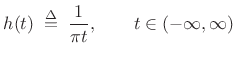
Hilbert Transform
The Hilbert transform ![]() of a real, continuous-time signal
of a real, continuous-time signal
![]() may be expressed as the convolution of
may be expressed as the convolution of ![]() with the
Hilbert transform kernel:
with the
Hilbert transform kernel:
That is, the Hilbert transform of
| (5.18) |
Thus, the Hilbert transform is a non-causal linear time-invariant filter.
The complex analytic signal ![]() corresponding to the real signal
corresponding to the real signal ![]() is
then given by
is
then given by
 |
(5.19) |
To show this last equality (note the lower limit of 0
instead of the
usual ![]() ), it is easiest to apply (4.16) in the frequency
domain:
), it is easiest to apply (4.16) in the frequency
domain:
| (5.20) | |||
| (5.21) |
Thus, the negative-frequency components of
Filtering and Windowing the Ideal
Hilbert-Transform Impulse Response
Let ![]() denote the convolution kernel of the continuous-time
Hilbert transform from (4.17) above:
denote the convolution kernel of the continuous-time
Hilbert transform from (4.17) above:

Convolving a real signal
Note that we cannot allow a time-domain sample at time 0 in (4.22) because it would be infinity. Instead, time 0 should be taken to lie between two samples, thereby introducing a small non-integer advance or delay. We'll choose a half-sample delay. As a result, we'll need to delay the real-part filter by half a sample as well when we make a complete single-sideband filter.
The matlab below illustrates the design of an FIR Hilbert-transform
filter by the window method using a Kaiser window. For a more
practical illustration, the sampling-rate assumed is set to
![]() Hz instead of being normalized to 1 as usual. The
Kaiser-window
Hz instead of being normalized to 1 as usual. The
Kaiser-window ![]() parameter is set to
parameter is set to ![]() , which normally gives
``pretty good'' audio performance (cf. Fig.3.28). From
Fig.3.28, we see that we can expect a stop-band attenuation
better than
, which normally gives
``pretty good'' audio performance (cf. Fig.3.28). From
Fig.3.28, we see that we can expect a stop-band attenuation
better than ![]() dB. The choice of
dB. The choice of ![]() , in setting the
time-bandwidth product of the Kaiser window, determines both the
stop-band rejection and the transition bandwidths required by our FIR
frequency response.
, in setting the
time-bandwidth product of the Kaiser window, determines both the
stop-band rejection and the transition bandwidths required by our FIR
frequency response.
  M = 257;    % window length = FIR filter length (Window Method)
  fs = 22050; % sampling rate assumed (Hz)
  f1 = 530;   % lower pass-band limit = transition bandwidth (Hz)
  beta = 8;   % beta for Kaiser window for decent side-lobe rejection
Recall that, for a rectangular window, our minimum transition bandwidth would be
Matlab, Continued
Given the above design parameters, we compute some derived parameters as follows:
  fn = fs/2;             % Nyquist limit (Hz)
  f2 = fn - f1;          % upper pass-band limit
  N = 2^(nextpow2(8*M)); % large FFT for interpolated display
  k1 = round(N*f1/fs);   % lower band edge in bins
  if k1<2, k1=2; end;    % cannot have dc or fn response
  kn = N/2 + 1;          % bin index at Nyquist limit (1-based)
  k2 = kn-k1+1;          % high-frequency band edge
  f1 = k1*fs/N           % quantized band-edge frequencies
  f2 = k2*fs/N
Setting the upper transition band the same as the low-frequency band (
Kaiser Window
With the filter length ![]() and Kaiser window
and Kaiser window ![]() as given
above, we may compute the Kaiser window itself in matlab via
as given
above, we may compute the Kaiser window itself in matlab via
w = kaiser(M,beta)'; % Kaiser window in "linear phase form"The spectrum of this window (zero-padded by more than a factor of 8) is shown in Fig.4.9 (full magnitude spectrum) and Fig.4.10 (zoom-in on the main lobe).
![\includegraphics[width=0.8\twidth]{eps/KaiserFR}](http://www.dsprelated.com/josimages_new/sasp2/img792.png)
![\includegraphics[width=0.8\twidth]{eps/KaiserZoomFR}](http://www.dsprelated.com/josimages_new/sasp2/img793.png)
Windowing a Desired Impulse Response Computed by the
Frequency Sampling Method
The next step is to apply our Kaiser window to the ``desired'' impulse
response, where ``desired'' means a time-shifted (by 1/2 sample) and
bandlimited (to introduce transition bands) version of the ``ideal''
impulse response in (4.22). In principle, we are using the
frequency-sampling method (§4.4) to prepare a
desired FIR filter of length ![]() as the inverse FFT of a desired
frequency response prepared by direct Fourier intuition. This long
FIR filter is then ``windowed'' down to length
as the inverse FFT of a desired
frequency response prepared by direct Fourier intuition. This long
FIR filter is then ``windowed'' down to length ![]() to give us our
final FIR filter designed by the window method.
to give us our
final FIR filter designed by the window method.
If the smallest transition bandwidth is ![]() Hz, then the FFT size
Hz, then the FFT size ![]() should satisfy
should satisfy
![]() . Otherwise, there may be too much time
aliasing in the desired impulse response.5.10 The only non-obvious
part in the matlab below is ``
. Otherwise, there may be too much time
aliasing in the desired impulse response.5.10 The only non-obvious
part in the matlab below is ``.^8'' which smooths the taper to
zero and looks better on a log magnitude scale. It would also make
sense to do a linear taper on a dB scale which corresponds to
an exponential taper to zero.
H = [ ([0:k1-2]/(k1-1)).^8,ones(1,k2-k1+1),...
      ([k1-2:-1:0]/(k1-1)).^8, zeros(1,N/2-1)];
Figure 4.11 shows our desired amplitude response so constructed.
![\includegraphics[width=0.8\twidth]{eps/hilbertFRIdeal}](http://www.dsprelated.com/josimages_new/sasp2/img796.png)
Now we inverse-FFT the desired frequency response to obtain the desired impulse response:
h = ifft(H); % desired impulse response
hodd = imag(h(1:2:N));     % This should be zero
ierr = norm(hodd)/norm(h); % Look at numerical round-off error
% Typical value: ierr = 4.1958e-15
% Also look at time aliasing:
aerr = norm(h(N/2-N/32:N/2+N/32))/norm(h);
% Typical value: 4.8300e-04
The real part of the desired impulse response is shown in Fig.4.12, and the imaginary part in Fig.4.13.
![\includegraphics[width=0.8\twidth]{eps/hilbertIRRealIdeal}](http://www.dsprelated.com/josimages_new/sasp2/img797.png)
![\includegraphics[width=0.8\twidth]{eps/hilbertIRImagIdeal}](http://www.dsprelated.com/josimages_new/sasp2/img798.png)
Now use the Kaiser window to time-limit the desired impulse response:
% put window in zero-phase form:
wzp = [w((M+1)/2:M), zeros(1,N-M), w(1:(M-1)/2)];
hw = wzp .* h; % single-sideband FIR filter, zero-centered
Hw = fft(hw);  % for results display: plot(db(Hw));
hh = [hw(N-(M-1)/2+1:N),hw(1:(M+1)/2)]; % caual FIR
% plot(db(fft([hh,zeros(1,N-M)]))); % freq resp plot
Figure 4.14 and Fig.4.15
show the normalized dB magnitude frequency response of our
final FIR filter consisting of the ![]() nonzero samples of
hw.
nonzero samples of
hw.
![\includegraphics[width=0.8\twidth]{eps/KaiserHilbertFR}](http://www.dsprelated.com/josimages_new/sasp2/img799.png)
![\includegraphics[width=0.8\twidth]{eps/KaiserHilbertZoomedFR}](http://www.dsprelated.com/josimages_new/sasp2/img800.png)
More General FIR Filter Design
We have looked at more than just FIR filter design by the window method and frequency-sampling technique. The general steps were
- Prepare a desired frequency-response that ``seems achievable''
- Inverse FFT
- Window the result (time-limit it)
- FFT that to see how it looks
Comparison to Optimal Chebyshev FIR Filter
Let's now compare the window-method design using the Kaiser window to the optimal equiripple FIR filter design given by the Remez multiple exchange algorithm.
Note, by the way, that many filter-design software functions, such as firpm have special modes for designing Hilbert-transform filters [224].
It turns out that the Remez exchange algorithm has convergence
problems for filters larger than a few hundred taps. Therefore, the
FIR filter length ![]() was chosen above to be small enough to work
out in this comparison. However, keep in mind that for very large
filter orders, the Remez exchange method may not be an option. There
are more recently developed methods for optimal Chebyshev FIR filter
design, using ``convex optimization'' techniques, that may continue to
work at very high orders
[218,22,153]. The fast nonparametric
methods discussed above (frequency sampling, window method) will work
fine at extremely high orders.
was chosen above to be small enough to work
out in this comparison. However, keep in mind that for very large
filter orders, the Remez exchange method may not be an option. There
are more recently developed methods for optimal Chebyshev FIR filter
design, using ``convex optimization'' techniques, that may continue to
work at very high orders
[218,22,153]. The fast nonparametric
methods discussed above (frequency sampling, window method) will work
fine at extremely high orders.
The following Matlab command will try to design the FIR Hilbert-transform filter of the desired length with the desired transition bands:
hri = firpm(M-1, [f1,f2]/fn, [1,1], [1], 'Hilbert');Instead, however, we will use a more robust method [228] which uses the Remez exchange algorithm to design a lowpass filter, followed by modulation of the lowpass impulse-response by a complex sinusoid at frequency
tic; % remember the current time
hrm = firpm(M-1, [0,(f2-fs/4)/fn,0.5,1], [1,1,0,0], [1,10]);
dt = toc; % design time dt can be minutes
hr = hrm .* j .^ [0:M-1]; % modulate lowpass to single-sideband
The weighting [1,10] in the call to firpm above says ``make the pass-band ripple
![\includegraphics[width=0.8\twidth]{eps/OptimalHilbertFR}](http://www.dsprelated.com/josimages_new/sasp2/img802.png) |
![\includegraphics[width=0.8\twidth]{eps/OptimalHilbertZoomedFR}](http://www.dsprelated.com/josimages_new/sasp2/img803.png)
In this case we did not normalize the peak amplitude response to 0 dB because it has a ripple peak of about 1 dB in the pass-band. Figure 4.18 shows a zoom-in on the pass-band ripple.
![\includegraphics[width=0.8\twidth]{eps/OptimalHilbertZoomedPB}](http://www.dsprelated.com/josimages_new/sasp2/img804.png)
Conclusions
We can note the following points regarding our single-sideband FIR filter design by means of direct Fourier intuition, frequency-sampling, and the window-method:
- The pass-band ripple is much smaller than 0.1 dB, which is
``over designed'' and therefore wasting of taps.
- The stop-band response ``droops'' which ``wastes'' filter taps
when stop-band attenuation is the only stop-band specification. In
other words, the first stop-band ripple drives the spec (
 dB),
while all higher-frequency ripples are over-designed. On the other
hand, a high-frequency ``roll-off'' of this nature is quite natural
in the frequency domain, and it corresponds to a ``smoother pulse''
in the time domain. Sometimes making the stop-band attenuation
uniform will cause small impulses at the beginning and end of
the impulse response in the time domain. (The pass-band and
stop-band ripple can ``add up'' under the inverse Fourier transform
integral.) Recall this impulsive endpoint phenomenon for the
Chebyshev window shown in Fig.3.33.
dB),
while all higher-frequency ripples are over-designed. On the other
hand, a high-frequency ``roll-off'' of this nature is quite natural
in the frequency domain, and it corresponds to a ``smoother pulse''
in the time domain. Sometimes making the stop-band attenuation
uniform will cause small impulses at the beginning and end of
the impulse response in the time domain. (The pass-band and
stop-band ripple can ``add up'' under the inverse Fourier transform
integral.) Recall this impulsive endpoint phenomenon for the
Chebyshev window shown in Fig.3.33.
- The pass-band is degraded by early roll-off. The pass-band edge
is not exactly in the desired place.
- The filter length can be thousands of taps long without running
into numerical failure. Filters this long are actually needed for
sampling rate conversion
[270,218].
We can also note some observations regarding the optimal Chebyshev version designed by the Remez multiple exchange algorithm:
- The stop-band is ideal, equiripple.
- The transition bandwidth is close to half that of the
window method. (We already knew our chosen transition bandwidth was
not ``tight'', but our rule-of-thumb based on the Kaiser-window
main-lobe width predicted only about
 % excess width.)
- The pass-band is ideal, though over-designed for static audio spectra.
- The computational design time is orders of magnitude larger
than that for window method.
- The design fails to converge for filters much longer than 256
taps. (Need to increase working precision or use a different
method to get longer optimal Chebyshev FIR filters.)
Generalized Window Method
Reiterating and expanding on points made in §4.6.3, often we need a filter with a frequency response that is not analytically known. An example is a graphic equalizer in which a user may manipulate sliders in a graphical user interface to control the gain in each of several frequency bands. From the foregoing, the following procedure, based in spirit on the window method (§4.5), can yield good results:
- Synthesize the desired frequency response as the
smoothest possible interpolation of the desired
frequency-response points. For example, in a graphic equalizer,
cubic splines [286] could be used to connect the
desired band gains.5.12
- If the desired frequency response is real (as in simple band
gains), either plan for a zero-phase filter in the end, or
synthesize a desired phase, such as linear phase or minimum phase
(see §4.8 below).
- Perform the inverse Fourier transform of the (sampled) desired
frequency response to obtain the desired impulse response.
- Plot an overlay of the desired impulse response and the window
to be applied, ensuring that the great majority of the signal energy
in the desired impulse response lies under the window to be used.
- Multiply by the window.
- Take an FFT (now with zero padding introduced by the window).
- Plot an overlay of the original desired response and the response retained after time-domain windowing, and verify that the specifications are within an acceptable range.
Minimum-Phase Filter Design
Above, we used the Hilbert transform to find the imaginary part of an analytic signal from its real part. A closely related application of the Hilbert transform is constructing a minimum phase [263] frequency response from an amplitude response.
Let
![]() denote a desired complex, minimum-phase frequency response
in the digital domain (
denote a desired complex, minimum-phase frequency response
in the digital domain (![]() plane):
plane):
 |
(5.23) |
and suppose we have only the amplitude response
 |
(5.24) |
Then the phase response
| (5.25) |
If
Minimum-Phase and Causal Cepstra
To show that a frequency response is minimum phase if and only if the
corresponding cepstrum is causal, we may take the log of the
corresponding transfer function, obtaining a sum of terms of the form
![]() for the zeros and
for the zeros and
![]() for the poles.
Since all poles and zeros of a minimum-phase system must be inside the
unit circle of the
for the poles.
Since all poles and zeros of a minimum-phase system must be inside the
unit circle of the ![]() plane, the Laurent expansion of all such terms
(the cepstrum) must be causal. In practice, as discussed in
[263], we may compute an approximate cepstrum as an inverse FFT
of the log spectrum, and make it causal by ``flipping'' the
negative-time cepstral coefficients around to positive time (adding
them to the positive-time coefficients). That is
plane, the Laurent expansion of all such terms
(the cepstrum) must be causal. In practice, as discussed in
[263], we may compute an approximate cepstrum as an inverse FFT
of the log spectrum, and make it causal by ``flipping'' the
negative-time cepstral coefficients around to positive time (adding
them to the positive-time coefficients). That is
![]() , for
, for
![]() and
and
![]() for
for ![]() .
This effectively inverts all unstable poles and all non-minimum-phase
zeros with respect to the unit circle. In other terms,
.
This effectively inverts all unstable poles and all non-minimum-phase
zeros with respect to the unit circle. In other terms,
![]() (if unstable), and
(if unstable), and
![]() (if
non-minimum phase).
(if
non-minimum phase).
The Laurent expansion of a differentiable function of a complex
variable can be thought of as a two-sided Taylor expansion,
i.e., it includes both positive and negative powers of ![]() , e.g.,
, e.g.,
| (5.26) |
In digital signal processing, a Laurent series is typically expanded about points on the unit circle in the
Optimal FIR Digital Filter Design
We now look briefly at the topic of optimal FIR filter design. We saw examples above of optimal Chebyshev designs (§4.5.2). and an oversimplified optimal least-squares design (§4.3). Here we elaborate a bit on optimality formulations under various error norms.
Lp norms
The ![]() norm of an
norm of an ![]() -dimensional vector (signal)
-dimensional vector (signal) ![]() is defined as
is defined as
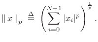 |
(5.27) |
Special Cases
 norm
norm

(5.28)
- Sum of the absolute values of the elements
- ``City block'' distance
 norm
norm
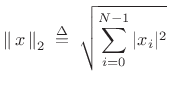
(5.29)
- ``Euclidean'' distance
- Minimized by ``Least Squares'' techniques
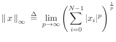
-
 norm
norm
In the limit as
 , the
, the  norm of
  is dominated by the maximum element of
. Optimal Chebyshev
filters minimize this norm of the frequency-response error.
is dominated by the maximum element of
. Optimal Chebyshev
filters minimize this norm of the frequency-response error.
Filter Design using Lp Norms
Formulated as an ![]() norm minimization, the FIR filter design problem
can be stated as follows:
norm minimization, the FIR filter design problem
can be stated as follows:
| (5.31) |
where
 FIR filter coefficients
-
 suitable discrete set of frequencies
-
 desired (complex) frequency response
-
 obtained frequency response (typically fft(h))
-
 (optional) error weighting function
Optimal Chebyshev FIR Filters
As we've seen above, the defining characteristic of FIR filters
optimal in the Chebyshev sense is that they minimize the maximum
frequency-response error-magnitude over the frequency axis. In
other terms, an optimal Chebyshev FIR filter is optimal in the
minimax sense: The filter coefficients are chosen to minimize
the worst-case error (maximum weighted error-magnitude ripple)
over all frequencies. This also means it is optimal in the
![]() sense because, as noted above, the
sense because, as noted above, the
![]() norm of a weighted
frequency-response error
norm of a weighted
frequency-response error
![]() is the maximum magnitude over all frequencies:
is the maximum magnitude over all frequencies:
| (5.32) |
Thus, we can say that an optimal Chebyshev filter minimizes the
The optimal Chebyshev FIR filter can often be found effectively using the Remez multiple exchange algorithm (typically called the Parks-McClellan algorithm when applied to FIR filter design) [176,224,66]. This was illustrated in §4.6.4 above. The Parks-McClellan/Remez algorithm also appears to be the most efficient known method for designing optimal Chebyshev FIR filters (as compared with, say linear programming methods using matlab's linprog as in §3.13). This algorithm is available in Matlab's Signal Processing Toolbox as firpm() (remez() in (Linux) Octave).5.13There is also a version of the Remez exchange algorithm for complex FIR filters. See §4.10.7 below for a few details.
The Remez multiple exchange algorithm has its limitations, however. In particular, convergence of the FIR filter coefficients is unlikely for FIR filters longer than a few hundred taps or so.
Optimal Chebyshev FIR filters are normally designed to be linear
phase [263] so that the desired frequency response
![]() can be taken to be real (i.e., first a zero-phase
FIR filter is designed). The design of linear-phase FIR filters in
the frequency domain can therefore be characterized as real
polynomial approximation on the unit circle [229,258].
can be taken to be real (i.e., first a zero-phase
FIR filter is designed). The design of linear-phase FIR filters in
the frequency domain can therefore be characterized as real
polynomial approximation on the unit circle [229,258].
In optimal Chebyshev filter designs, the error exhibits an
equiripple characteristic--that is, if the desired
response is ![]() and the ripple magnitude is
and the ripple magnitude is ![]() , then
the frequency response of the optimal FIR filter (in the unweighted
case, i.e.,
, then
the frequency response of the optimal FIR filter (in the unweighted
case, i.e.,
![]() for all
for all ![]() ) will oscillate between
) will oscillate between
![]() and
and
![]() as
as ![]() increases.
The powerful alternation theorem characterizes optimal
Chebyshev solutions in terms of the alternating error peaks.
Essentially, if one finds sufficiently many for the given FIR filter
order, then you have found the unique optimal Chebyshev solution
[224]. Another remarkable result is that the Remez
multiple exchange converges monotonically to the unique optimal
Chebyshev solution (in the absence of numerical round-off errors).
increases.
The powerful alternation theorem characterizes optimal
Chebyshev solutions in terms of the alternating error peaks.
Essentially, if one finds sufficiently many for the given FIR filter
order, then you have found the unique optimal Chebyshev solution
[224]. Another remarkable result is that the Remez
multiple exchange converges monotonically to the unique optimal
Chebyshev solution (in the absence of numerical round-off errors).
Fine online introductions to the theory and practice of Chebyshev-optimal FIR filter design are given in [32,283].
The window method (§4.5) and Remez-exchange method together span many practical FIR filter design needs, from ``quick and dirty'' to essentially ideal FIR filters (in terms of conventional specifications).
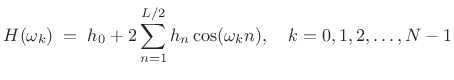
Least-Squares Linear-Phase FIR Filter Design
Another versatile, effective, and often-used case is the weighted least squares method, which is implemented in the matlab function firls and others. A good general reference in this area is [204].
Let the FIR filter length be ![]() samples, with
samples, with ![]() even, and suppose
we'll initially design it to be centered about the time origin (``zero
phase''). Then the frequency response is given on our frequency grid
even, and suppose
we'll initially design it to be centered about the time origin (``zero
phase''). Then the frequency response is given on our frequency grid
![]() by
by
 |
(5.33) |
Enforcing even symmetry in the impulse response, i.e.,
 |
(5.34) |
or, in matrix form:
![$\displaystyle \underbrace{\left[ \begin{array}{c} H(\omega_0) \\ H(\omega_1) \\ \vdots \\ H(\omega_{N-1}) \end{array} \right]}_{{\underline{d}}} = \underbrace{\left[ \begin{array}{ccccc} 1 & 2\cos(\omega_0) & \dots & 2\cos[\omega_0(L/2)] \\ 1 & 2\cos(\omega_1) & \dots & 2\cos[\omega_1(L/2)] \\ \vdots & \vdots & & \vdots \\ 1 & 2\cos(\omega_{N-1}) & \dots & 2\cos[\omega_{N-1}(L/2)] \end{array} \right]}_\mathbf{A} \underbrace{\left[ \begin{array}{c} h_0 \\ h_1 \\ \vdots \\ h_{L/2} \end{array} \right]}_{{\underline{h}}} \protect$](http://www.dsprelated.com/josimages_new/sasp2/img849.png)
Recall from §3.13.8, that the Remez multiple exchange
algorithm is based on this formulation internally. In that case, the
left-hand-side includes the alternating error, and the frequency grid
![]() iteratively seeks the frequencies of maximum error--the
so-called extremal frequencies.
iteratively seeks the frequencies of maximum error--the
so-called extremal frequencies.
In matrix notation, our filter-design problem can be stated as (cf. §3.13.8)
| (5.36) |
where these quantities are defined in (4.35). We can denote the optimal least-squares solution by
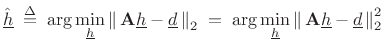 |
(5.37) |
To find
This is a quadratic form in
| (5.39) |
with solution
![$\displaystyle \zbox {{\underline{\hat{h}}}\eqsp \left[(\mathbf{A}^T\mathbf{A})^{-1}\mathbf{A}^T\right]{\underline{d}}.}$](http://www.dsprelated.com/josimages_new/sasp2/img859.png) |
(5.40) |
The matrix
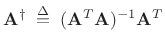 |
(5.41) |
is known as the (Moore-Penrose) pseudo-inverse of the matrix
Geometric Interpretation of Least Squares
Typically, the number of frequency constraints is much greater than the number of design variables (filter coefficients). In these cases, we have an overdetermined system of equations (more equations than unknowns). Therefore, we cannot generally satisfy all the equations, and are left with minimizing some error criterion to find the ``optimal compromise'' solution.
In the case of least-squares approximation, we are minimizing the Euclidean distance, which suggests the geometrical interpretation shown in Fig.4.19.
![\begin{psfrags}
% latex2html id marker 14494\psfrag{Ax}{{\Large $\mathbf{A}{\underline{\hat{h}}}$}}\psfrag{b}{{\Large ${\underline{d}}$}}\psfrag{column}{{\Large column-space of $\mathbf{A}$}}\psfrag{space}{}\begin{figure}[htbp]
\includegraphics[width=3in]{eps/lsq}
\caption{Geometric interpretation of orthogonal
projection of the vector ${\underline{d}}$\ onto the column-space of $\mathbf{A}$.}
\end{figure}
\end{psfrags}](http://www.dsprelated.com/josimages_new/sasp2/img862.png)
Thus, the desired vector
![]() is the vector sum of its
best least-squares approximation
is the vector sum of its
best least-squares approximation
![]() plus an orthogonal error
plus an orthogonal error ![]() :
:
| (5.42) |
In practice, the least-squares solution
| (5.43) |
Figure 4.19 suggests that the error vector
| (5.44) |
This is how the orthogonality principle can be used to derive the fact that the best least squares solution is given by
| (5.45) |
In matlab, it is numerically superior to use ``h= A
We will return to least-squares optimality in §5.7.1 for the purpose of estimating the parameters of sinusoidal peaks in spectra.
Matlab Support for Least-Squares FIR Filter Design
Some of the available functions are as follows:
- firls - least-squares linear-phase FIR filter design
for piecewise constant desired amplitude responses -- also designs
Hilbert transformers and differentiators
- fircls - constrained least-squares linear-phase FIR
filter design for piecewise constant desired amplitude responses --
constraints provide lower and upper bounds on the frequency response
- fircls1 - constrained least-squares linear-phase FIR
filter design for lowpass and highpass filters -- supports relative
weighting of pass-band and stop-band error
For more information, type help firls and/or doc firls, etc., and refer to the ``See Also'' section of the documentation for pointers to more relevant functions.
Chebyshev FIR Design via Linear Programming
We return now to the
![]() -norm minimization problem of §4.10.2:
-norm minimization problem of §4.10.2:
and discuss its formulation as a linear programming problem, very similar to the optimal window formulations in §3.13. We can rewrite (4.46) as
| (5.47) |
where
| s.t. | (5.48) |
Introducing a new variable
![$\displaystyle \tilde{{\underline{h}}} \isdefs \left[ \begin{array}{c} {\underline{h}}\\ t \end{array} \right],$](http://www.dsprelated.com/josimages_new/sasp2/img876.png) |
(5.49) |
then we can write
![$\displaystyle t \eqsp f^T \tilde{{\underline{h}}} \isdefs \left[\begin{array}{cccc} 0 & \cdots & 0 & 1 \end{array}\right] \tilde{{\underline{h}}},$](http://www.dsprelated.com/josimages_new/sasp2/img877.png) |
(5.50) |
and our optimization problem can be written in more standard form:
| s.t. | ![$\displaystyle \left\vert [\begin{array}{cc} a_k^T \; 0\\ \end{array} ] \cdot \tilde{{\underline{h}}} -{\underline{d}}_k \right\vert
\;<\; \tilde{{\underline{h}}}^T f^T\tilde{{\underline{h}}}$](http://www.dsprelated.com/josimages_new/sasp2/img880.png) |
(5.51) |
Thus, we are minimizing a linear objective, subject to a set of linear inequality constraints. This is known as a linear programming problem, as discussed previously in §3.13.1, and it may be solved using the matlab linprog function. As in the case of optimal window design, linprog is not normally as efficient as the Remez multiple exchange algorithm (firpm), but it is more general, allowing for linear equality and inequality constraints to be imposed.
More General Real FIR Filters
So far we have looked at the design of linear phase filters. In this
case,
![]() ,
,
![]() and
and
![]() are all real. In some
applications, we need to specify both the magnitude and
phase of the frequency response. Examples include
are all real. In some
applications, we need to specify both the magnitude and
phase of the frequency response. Examples include
- minimum phase filters [263],
- inverse filters (``deconvolution''),
- fractional delay filters [266],
- interpolation polyphase subfilters (Chapter 11)
Nonlinear-Phase FIR Filter Design
Above, we considered only linear-phase (symmetric) FIR filters. The same methods also work for antisymmetric FIR filters having a purely imaginary frequency response, when zero-centered, such as differentiators and Hilbert transformers [224].
We now look at extension to nonlinear-phase FIR filters,
managed by treating the real and imaginary parts separately in the
frequency domain [218]. In the
nonlinear-phase case, the frequency response is complex in
general. Therefore, in the formulation Eq.![]() (4.35) both
(4.35) both
![]() and
and
![]() are complex, but we still desire the FIR filter coefficients
are complex, but we still desire the FIR filter coefficients
![]() to be real. If we try to use '
to be real. If we try to use '
![]() ' or pinv in
matlab, we will generally get a complex result for
' or pinv in
matlab, we will generally get a complex result for
![]() .
.
Problem Formulation
| (5.52) |
where
| (5.53) |
which can be written as
| (5.54) |
or
![$\displaystyle \min_{\underline{h}}\left\vert \left\vert \left[ \begin{array}{c} {\cal{R}}(\mathbf{A}) \\ {\cal{I}}(\mathbf{A}) \end{array} \right] {\underline{h}} - \left[ \begin{array}{c} {\cal{R}}({\underline{d}}) \\ {\cal{I}}({\underline{d}}) \end{array}\right] \right\vert \right\vert _2^2$](http://www.dsprelated.com/josimages_new/sasp2/img887.png) |
(5.55) |
which is written in terms of only real variables.
In summary, we can use the standard least-squares solvers in matlab and end up with a real solution for the case of complex desired spectra and nonlinear-phase FIR filters.
Matlab for General FIR Filter Design
The cfirpm function (formerly cremez)
[116,117] in the Matlab Signal
Processing Toolbox performs complex
![]() FIR filter design
(``Complex FIR Parks-McClellan''). Convergence is theoretically
guaranteed for arbitrary magnitude and phase specifications
versus frequency. It reduces to Parks-McClellan algorithm (Remez
second algorithm) as a special case.
FIR filter design
(``Complex FIR Parks-McClellan''). Convergence is theoretically
guaranteed for arbitrary magnitude and phase specifications
versus frequency. It reduces to Parks-McClellan algorithm (Remez
second algorithm) as a special case.
The firgr function (formerly gremez) in the Matlab
Filter Design Toolbox performs ``generalized''
![]() FIR filter
design, adding support for minimum-phase FIR filter design, among
other features [254].
FIR filter
design, adding support for minimum-phase FIR filter design, among
other features [254].
Finally, the fircband function in the Matlab DSP System Toolbox designs a variety of real FIR filters with various filter-types and constraints supported.
This is of course only a small sampling of what is available. See, e.g., the Matlab documentation on its various toolboxes relevant to filter design (especially the Signal Processing and Filter Design toolboxes) for much more.
Second-Order Cone Problems
In Second-Order Cone Problems (SOCP), a linear function is minimized over the intersection of an affine set and the product of second-order (quadratic) cones [153,22]. Nonlinear, convex problem including linear and (convex) quadratic programs are special cases. SOCP problems are solved by efficient primal-dual interior-point methods. The number of iterations required to solve a problem grows at most as the square root of the problem size. A typical number of iterations ranges between 5 and 50, almost independent of the problem size.
Resources
- LIPSOL: Matlab code for linear programming using interior point methods.
- Matlab's linprog (in the Optimization Toolbox)
- Octave's lp (SourceForge package)
Nonlinear Optimization in Matlab
There are various matlab functions available for nonlinear optimizations as well. These can be utilized in more exotic FIR filter designs, such as designs driven more by perceptual criteria:
- The fsolve function in Octave, or the Matlab Optimization Toolbox, attempts to solve unconstrained, overdetermined, nonlinear systems of equations.
- The Octave function sqp handles constrained nonlinear optimization.
- The Octave optim package includes many additional functions such as leasqr for performing Levenberg-Marquardt nonlinear regression. (Say, e.g., which leasqr and explore its directory.)
- The Matlab Optimization Toolbox similarly contains many functions for optimization.
Next Section:
Spectrum Analysis of Sinusoids
Previous Section:
Spectrum Analysis Windows


