


Perfect Reconstruction Filter Banks
We now consider filter banks with an arbitrary number of channels, and
ask under what conditions do we obtain a perfect reconstruction filter
bank? Polyphase analysis will give us the answer readily. Let's
begin with the ![]() -channel filter bank in Fig.11.20. The
downsampling factor is
-channel filter bank in Fig.11.20. The
downsampling factor is ![]() . For critical sampling, we set
. For critical sampling, we set
![]() .
.
![\includegraphics[width=\twidth]{eps/FBNchan}](http://www.dsprelated.com/josimages_new/sasp2/img2096.png)
The next step is to expand each analysis filter ![]() into its
into its
![]() -channel ``type I'' polyphase representation:
-channel ``type I'' polyphase representation:
 |
(12.49) |
or
![$\displaystyle \underbrace{\left[\begin{array}{c} H_0(z) \\ [2pt] H_1(z) \\ [2pt] \vdots \\ [2pt] \!\!H_{N-1}(z)\!\!\end{array}\right]}_{\bold{h}(z)} = \underbrace{\left[\begin{array}{cccc} E_{0,0}(z^N) & E_{0,1}(z^N) & \cdots & E_{0,N-1}(z^N) \\ E_{1,0}(z^N) & E_{1,1}(z^N) & \cdots & E_{1,N-1}(z^N)\\ \vdots & \vdots & \cdots & \vdots\\ \!\!E_{N-1,0}(z^N) & E_{N-1,1}(z^N) & \cdots & E_{N-1,N-1}(z^N) \!\! \end{array}\right]}_{\bold{E}(z^N)} \underbrace{\left[\begin{array}{c} 1 \\ [2pt] z^{-1} \\ [2pt] \vdots \\ [2pt] \!\!z^{-(N-1)}\!\!\end{array}\right]}_{\bold{e}(z)}$](http://www.dsprelated.com/josimages_new/sasp2/img2099.png) |
(12.50) |
which we can write as
| (12.51) |
Similarly, expand the synthesis filters in a type II polyphase decomposition:
 |
(12.52) |
or
![$\displaystyle \underbrace{\left[\begin{array}{c} F_0(z) \\ [2pt] F_1(z) \\ [2pt] \vdots \\ [2pt] \!\!F_{N-1}(z)\!\!\end{array}\right]^T}_{\bold{f}^T(z)} \eqsp \underbrace{\left[\begin{array}{c} \!\!z^{-(N-1)}\!\! \\ [2pt] \!\!z^{-(N-2)}\!\! \\ [2pt] \vdots \\ [2pt] 1\end{array}\right]^T}_{{\tilde{\bold{e}}}(z)} \underbrace{\left[\begin{array}{cccc} R_{0,0}(z^N) & R_{0,1}(z^N) & \cdots & R_{0,N-1}(z^N) \\ R_{1,0}(z^N) & R_{1,1}(z^N) & \cdots & R_{1,N-1}(z^N)\\ \vdots & \vdots & \cdots & \vdots\\ \!\!R_{N-1,0}(z^N) & R_{N-1,1}(z^N) & \cdots & R_{N-1,N-1}(z^N)\!\! \end{array}\right]}_{\bold{R}(z^N)}$](http://www.dsprelated.com/josimages_new/sasp2/img2102.png) |
(12.53) |
which we can write as
| (12.54) |
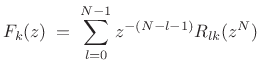
The polyphase representation can now be depicted as shown in
Fig.11.21. When ![]() , commuting the up/downsamplers gives
the result shown in Fig.11.22. We call
, commuting the up/downsamplers gives
the result shown in Fig.11.22. We call
![]() the
polyphase matrix.
the
polyphase matrix.
![\includegraphics[width=\twidth]{eps/polyNchan}](http://www.dsprelated.com/josimages_new/sasp2/img2105.png)
![\includegraphics[width=\twidth]{eps/polyNchanfast}](http://www.dsprelated.com/josimages_new/sasp2/img2106.png)
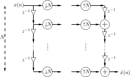
As we will show below, the above simplification can be carried out
more generally whenever ![]() divides
divides ![]() (e.g.,
(e.g.,
![]() ). In these cases
). In these cases
![]() becomes
becomes
![]() and
and
![]() becomes
becomes
![]() .
.
Simple Examples of Perfect Reconstruction
If we can arrange to have
| (12.55) |
then the filter bank will reduce to the simple system shown in Fig.11.23.
Thus, when ![]() and
and
![]() ,
we have a simple parallelizer/serializer,
which is perfect-reconstruction by inspection: Referring to
Fig.11.23, think of the input samples
,
we have a simple parallelizer/serializer,
which is perfect-reconstruction by inspection: Referring to
Fig.11.23, think of the input samples ![]() as ``filling'' a
length
as ``filling'' a
length ![]() delay line over
delay line over ![]() sample clocks. At time 0
, the
downsamplers and upsamplers ``fire'', transferring
sample clocks. At time 0
, the
downsamplers and upsamplers ``fire'', transferring ![]() (and
(and ![]() zeros) from the delay line to the output delay chain, summing with
zeros. Over the next
zeros) from the delay line to the output delay chain, summing with
zeros. Over the next ![]() clocks,
clocks, ![]() makes its way toward the
output, and zeros fill in behind it in the output delay chain.
Simultaneously, the input buffer is being filled with samples of
makes its way toward the
output, and zeros fill in behind it in the output delay chain.
Simultaneously, the input buffer is being filled with samples of
![]() . At time
. At time ![]() ,
, ![]() makes it to the output. At time
makes it to the output. At time ![]() ,
the downsamplers ``fire'' again, transferring a length
,
the downsamplers ``fire'' again, transferring a length ![]() ``buffer''
[
``buffer''
[![]() :
:![]() ] to the upsamplers. On the same clock pulse, the
upsamplers also ``fire'', transferring
] to the upsamplers. On the same clock pulse, the
upsamplers also ``fire'', transferring ![]() samples to the output delay
chain. The bottom-most sample [
samples to the output delay
chain. The bottom-most sample [
![]() ] goes out immediately
at time
] goes out immediately
at time ![]() . Over the next
. Over the next ![]() sample clocks, the length
sample clocks, the length ![]() output buffer will be ``drained'' and refilled by zeros.
Simultaneously, the input buffer will be replaced by new samples of
output buffer will be ``drained'' and refilled by zeros.
Simultaneously, the input buffer will be replaced by new samples of
![]() . At time
. At time ![]() , the downsamplers and upsamplers ``fire'', and
the process goes on, repeating with period
, the downsamplers and upsamplers ``fire'', and
the process goes on, repeating with period ![]() . The output of the
. The output of the
![]() -way parallelizer/serializer is therefore
-way parallelizer/serializer is therefore
| (12.56) |
and we have perfect reconstruction.
Sliding Polyphase Filter Bank
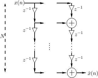
When ![]() , there is no downsampling or upsampling, and the system
further reduces to the case shown in Fig.11.24. Working
backward along the output delay chain, the output sum can be written
as
, there is no downsampling or upsampling, and the system
further reduces to the case shown in Fig.11.24. Working
backward along the output delay chain, the output sum can be written
as
![\begin{eqnarray*}
\hat{X}(z) &=& \left[z^{-0}z^{-(N-1)} + z^{-1}z^{-(N-2)} + z^{-2}z^{-(N-3)} + \cdots \right.\\
& & \left. + z^{-(N-2)}z^{-1} + z^{-(N-1)}z^{-0} \right] X(z)\\
&=& N z^{-(N-1)} X(z).
\end{eqnarray*}](http://www.dsprelated.com/josimages_new/sasp2/img2121.png)
Thus, when ![]() , the output is
, the output is
| (12.57) |
and we again have perfect reconstruction.
Hopping Polyphase Filter Bank
When ![]() and
and ![]() divides
divides ![]() , we have, by a similar analysis,
, we have, by a similar analysis,
 |
(12.58) |
which is again perfect reconstruction. Note the built-in overlap-add when
Sufficient Condition for Perfect Reconstruction
Above, we found that, for any integer
![]() which divides
which divides
![]() , a sufficient condition for perfect reconstruction is
, a sufficient condition for perfect reconstruction is
 |
(12.59) |
and the output signal is then
 |
(12.60) |
More generally, we allow any nonzero scaling and any additional delay:
where
 |
(12.62) |
Thus, given any polyphase matrix
![]() , we can attempt to compute
, we can attempt to compute
![]() : If it is stable, we can use it to build a
perfect-reconstruction filter bank. However, if
: If it is stable, we can use it to build a
perfect-reconstruction filter bank. However, if
![]() is FIR,
is FIR,
![]() will typically be IIR. In §11.5 below, we will look at
paraunitary filter banks, for which
will typically be IIR. In §11.5 below, we will look at
paraunitary filter banks, for which
![]() is FIR and
paraunitary whenever
is FIR and
paraunitary whenever
![]() is.
is.
Necessary and Sufficient Conditions for Perfect Reconstruction
It can be shown [287] that the most general conditions for perfect reconstruction are that
![$\displaystyle \zbox {\bold{R}(z)\bold{E}(z) \eqsp c z^{-K} \left[\begin{array}{cc} \bold{0}_{(N-L)\times L} & z^{-1}\bold{I}_{N-L} \\ [2pt] \bold{I}_L & \bold{0}_{L \times (N-L)} \end{array}\right]}$](http://www.dsprelated.com/josimages_new/sasp2/img2132.png) |
(12.63) |
for some constant
Note that the more general form of
![]() above can be regarded as a (non-unique) square root of a vector unit delay, since
above can be regarded as a (non-unique) square root of a vector unit delay, since
![$\displaystyle \left[\begin{array}{cc} \bold{0}_{(N-L)\times L} & z^{-1}\bold{I}_{N-L} \\ [2pt] \bold{I}_L & \bold{0}_{L \times (N-L)} \end{array}\right]^2 \eqsp z^{-1}\bold{I}_N.$](http://www.dsprelated.com/josimages_new/sasp2/img2136.png) |
(12.64) |
Thus, the general case is the same thing as
| (12.65) |
except for some channel swapping and an extra sample of delay in some channels.
Polyphase View of the STFT
As a familiar special case, set
| (12.66) |
where
![$\displaystyle \bold{W}_N^\ast[kn] \eqsp \left[e^{-j2\pi kn/N}\right]$](http://www.dsprelated.com/josimages_new/sasp2/img2140.png) |
(12.67) |
The inverse of this polyphase matrix is then simply the inverse DFT matrix:
 |
(12.68) |
Thus, the STFT (with rectangular window) is the simple special case of a perfect reconstruction filter bank for which the polyphase matrix is constant. It is also unitary; therefore, the STFT is an orthogonal filter bank.
The channel analysis and synthesis filters are, respectively,
![\begin{eqnarray*}
H_k(z) &=& H_0(zW_N^k)\\ [5pt]
F_k(z) &=& F_0(zW_N^{-k})
\end{eqnarray*}](http://www.dsprelated.com/josimages_new/sasp2/img2142.png)
where
 , and
, and
![$\displaystyle F_0(z)\eqsp H_0(z)\eqsp \sum_{n=0}^{N-1}z^{-n}\;\longleftrightarrow\;[1,1,\ldots,1]$](http://www.dsprelated.com/josimages_new/sasp2/img2144.png) |
(12.69) |
corresponding to the rectangular window.
![\includegraphics[width=\twidth]{eps/polyNchanSTFT}](http://www.dsprelated.com/josimages_new/sasp2/img2145.png)
Looking again at the polyphase representation of the ![]() -channel
filter bank with hop size
-channel
filter bank with hop size ![]() ,
,
![]() ,
,
![]() ,
,
![]() dividing
dividing ![]() , we have the system shown in Fig.11.25.
Following the same analysis as in §11.4.1 leads to the following
conclusion:
, we have the system shown in Fig.11.25.
Following the same analysis as in §11.4.1 leads to the following
conclusion:
Our analysis showed that the STFT using a rectangular window is
a perfect reconstruction filter bank for all
integer hop sizes in the set
![]() .
The same type of analysis can be applied to the STFT using the other
windows we've studied, including Portnoff windows.
.
The same type of analysis can be applied to the STFT using the other
windows we've studied, including Portnoff windows.
Example: Polyphase Analysis of the STFT with 50% Overlap, Zero-Padding, and a Non-Rectangular Window
![\includegraphics[width=\twidth]{eps/polyNchanWinZPSTFT}](http://www.dsprelated.com/josimages_new/sasp2/img2150.png)
Figure 11.26 illustrates how a window and a hop size other than
![]() can be introduced into the polyphase representation of the STFT.
The constant-overlap-add of the window
can be introduced into the polyphase representation of the STFT.
The constant-overlap-add of the window ![]() is implemented in the
synthesis delay chain (which is technically the
transpose of a tapped delay
line). The downsampling factor and window must be selected
together to give constant overlap-add, independent of the
choice of polyphase matrices
is implemented in the
synthesis delay chain (which is technically the
transpose of a tapped delay
line). The downsampling factor and window must be selected
together to give constant overlap-add, independent of the
choice of polyphase matrices
![]() and
and
![]() (shown here as the
(shown here as the
![]() and
and
![]() ).
).
Example: Polyphase Analysis of the Weighted Overlap Add Case: 50% Overlap, Zero-Padding, and a Non-Rectangular Window
We may convert the previous example to a weighted overlap-add
(WOLA) (§8.6) filter bank by replacing each ![]() by
by
![]() and introducing these gains also between the
and introducing these gains also between the
![]() and
upsamplers, as shown in Fig.11.27.
and
upsamplers, as shown in Fig.11.27.
![\includegraphics[width=\twidth]{eps/polyNchanWinZPWOLA}](http://www.dsprelated.com/josimages_new/sasp2/img2155.png)
Next Section:
Paraunitary Filter Banks
Previous Section:
Critically Sampled Perfect Reconstruction Filter Banks


