


Sinusoidal Amplitude Estimation
If the sinusoidal frequency ![]() and phase
and phase ![]() happen to be
known, we obtain a simple linear least squares problem for the
amplitude
happen to be
known, we obtain a simple linear least squares problem for the
amplitude ![]() . That is, the error signal
. That is, the error signal
| (6.36) |
becomes linear in the unknown parameter
becomes a simple quadratic (parabola) over the real line.6.11 Quadratic forms in any number of dimensions are easy to minimize. For example, the ``bottom of the bowl'' can be reached in one step of Newton's method. From another point of view, the optimal parameter
Yet a third way to minimize (5.37) is the method taught in
elementary calculus: differentiate
![]() with respect to
with respect to ![]() , equate
it to zero, and solve for
, equate
it to zero, and solve for ![]() . In preparation for this, it is helpful to
write (5.37) as
. In preparation for this, it is helpful to
write (5.37) as
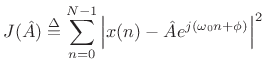
![\begin{eqnarray*}
J({\hat A}) &\isdef & \sum_{n=0}^{N-1}
\left[x(n)-{\hat A}e^{j(\omega_0 n+\phi)}\right]
\left[\overline{x(n)}-\overline{{\hat A}} e^{-j(\omega_0 n+\phi)}\right]\\
&=&
\sum_{n=0}^{N-1}
\left[
\left\vert x(n)\right\vert^2
-
x(n)\overline{{\hat A}} e^{-j(\omega_0 n+\phi)}
-
\overline{x(n)}{\hat A}e^{j(\omega_0 n+\phi)}
+
{\hat A}^2
\right]
\\
&=& \left\Vert\,x\,\right\Vert _2^2 - 2\mbox{re}\left\{\sum_{n=0}^{N-1} x(n)\overline{{\hat A}}
e^{-j(\omega_0 n+\phi)}\right\}
+ N {\hat A}^2.
\end{eqnarray*}](http://www.dsprelated.com/josimages_new/sasp2/img1045.png)
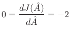
Differentiating with respect to ![]() and equating to zero yields
and equating to zero yields
 re re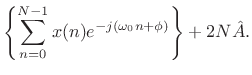 |
(6.38) |
Solving this for
 re
re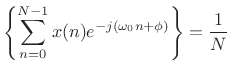 re
reThat is, the optimal least-squares amplitude estimate may be found by the following steps:
- Multiply the data
 by
by
 to zero the known phase
  .
.
- Take the DFT of the
 samples of
  , suitably zero padded to approximate the DTFT, and evaluate it at the known frequency
  .
.
- Discard any imaginary part since it can only contain noise, by (5.39).
- Divide by
to obtain a properly normalized coefficient of projection
[264] onto the sinusoid
(6.40)
Next Section:
Sinusoidal Amplitude and Phase Estimation
Previous Section:
Matlab for Computing Minimum Zero-Padding Factors


