


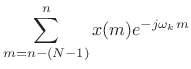
Uniform Running-Sum Filter Banks
Using a length ![]() running-sum filter, let's make
running-sum filter, let's make ![]() bandpass filters
tuned to center frequencies
bandpass filters
tuned to center frequencies
 |
(10.11) |
Since the bandwidths, as defined, are
![\includegraphics[width=3in]{eps/sincbank}](http://www.dsprelated.com/josimages_new/sasp2/img1591.png)
System Diagram of the Running-Sum Filter Bank
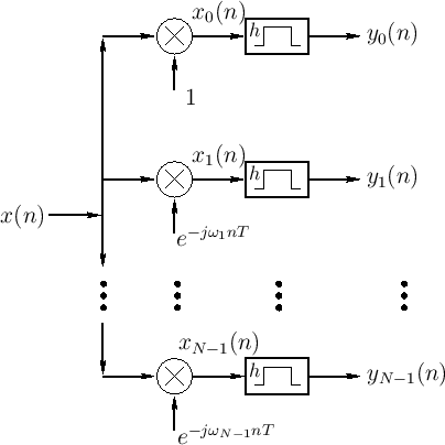
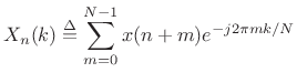
Figure 9.15 shows the system diagram of the complete ![]() -channel filter bank
constructed using length
-channel filter bank
constructed using length ![]() FIR running-sum lowpass filters. The
FIR running-sum lowpass filters. The
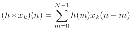
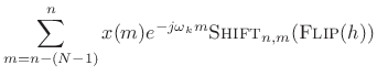
![]() th channel computes:
th channel computes:

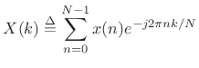
DFT Filter Bank
Recall that the Length ![]() Discrete Fourier Transform (DFT) is
defined as
Discrete Fourier Transform (DFT) is
defined as
 |
(10.13) |
Comparing this to (9.12), we see that the filter-bank output
| (10.14) |
In other words, the filter-bank output at time
More generally, for all ![]() , we will call Fig.9.15 the DFT
filter bank. The DFT filter bank is the special case of the STFT for
which a rectangular window and hop size
, we will call Fig.9.15 the DFT
filter bank. The DFT filter bank is the special case of the STFT for
which a rectangular window and hop size ![]() are used.
are used.
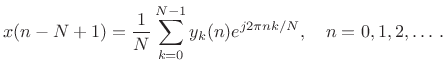
The sliding DFT is obtained by advancing successive DFTs by one sample:
 |
(10.15) |
When
When ![]() is a power of 2, the DFT can be implemented using a Cooley-Tukey Fast
Fourier Transform (FFT) using only
is a power of 2, the DFT can be implemented using a Cooley-Tukey Fast
Fourier Transform (FFT) using only
![]() operations per
transform. By keeping track of the linear phase term (an
operations per
transform. By keeping track of the linear phase term (an
![]() modification), a DFT Filter Bank can be implemented efficiently using
an FFT. Uniform FIR filter banks are very often implemented in
practice using FFT software such as fftw.
modification), a DFT Filter Bank can be implemented efficiently using
an FFT. Uniform FIR filter banks are very often implemented in
practice using FFT software such as fftw.
Note that the channel bandwidths are narrow compared with half
the sampling rate (especially for large ![]() ), so that the filter bank
output signals
), so that the filter bank
output signals ![]() are oversampled, in general. We will
later look at downsampling the channel signals
are oversampled, in general. We will
later look at downsampling the channel signals ![]() to
obtain a ``hopping FFT'' filter bank. ``Sliding'' and ``hopping''
FFTs are special cases of the discrete-time Short Time Fourier
Transform (STFT). The STFT normally also uses a window
function other than the rectangular window used in this development
(the running-sum lowpass filter).
to
obtain a ``hopping FFT'' filter bank. ``Sliding'' and ``hopping''
FFTs are special cases of the discrete-time Short Time Fourier
Transform (STFT). The STFT normally also uses a window
function other than the rectangular window used in this development
(the running-sum lowpass filter).
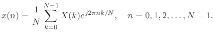
Inverse DFT and the DFT Filter Bank Sum
The Length ![]() inverse DFT is given by [264]
inverse DFT is given by [264]
 |
(10.16) |
This suggests that the DFT Filter Bank can be inverted by simply remodulating the baseband filter-bank signals
 |
(10.17) |
This is in fact true, as we will later see. (It is straightforward to show as an exercise.)
Specific Windows
- Recall that the rectangular window transform is
 , implying the rectangular window itself is
 ,
which is obvious.
,
which is obvious.
- The window transform for the Hamming family is
 ,
implying that Hamming windows are
,
implying that Hamming windows are
 , which we also knew.
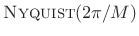
- The rectangular window transform is also
 for any integer
 , implying that all hop sizes given
by
, implying that all hop sizes given
by  for
for
 are COLA.
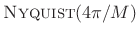
- Because its side lobes are the same width as the sinc side lobes,
the Hamming window transform is also
,for any integer
 , implying hop sizes
are good, for
, implying hop sizes
are good, for
 . Thus, the available hop sizes for the Hamming
window family include all of those for the rectangular window
except one (
. Thus, the available hop sizes for the Hamming
window family include all of those for the rectangular window
except one ( ).
).
The Nyquist Property on the Unit Circle
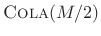
As a degenerate case, note that ![]() is COLA for any window, while no
window transform is
is COLA for any window, while no
window transform is
![]() except the zero window. (since it
would have to be zero at dc, and we do not consider such windows).
Did the theory break down for
except the zero window. (since it
would have to be zero at dc, and we do not consider such windows).
Did the theory break down for ![]() ?
?
Intuitively, the
![]() condition on the window transform
condition on the window transform
![]() ensures that all nonzero multiples of the
time-domain-frame-rate
ensures that all nonzero multiples of the
time-domain-frame-rate ![]() will be zeroed out over the interval
will be zeroed out over the interval
![]() along the frequency axis. When the frame-rate equals the
sampling rate (
along the frequency axis. When the frame-rate equals the
sampling rate (![]() ), there are no frame-rate multiples in the
range
), there are no frame-rate multiples in the
range
![]() . (The range
. (The range ![]() gives the same result.)
When
gives the same result.)
When ![]() , there is exactly one frame-rate multiple at
, there is exactly one frame-rate multiple at ![]() . When
. When
![]() , there are two at
, there are two at
![]() . When
. When ![]() , they are at
, they are at ![]() and
and ![]() , and so on.
, and so on.
We can cleanly handle the special case of ![]() by defining all
functions over the unit circle as being
by defining all
functions over the unit circle as being
![]() when there are no
frame-rate multiples in the range
when there are no
frame-rate multiples in the range
![]() . Thus, a discrete-time
spectrum
. Thus, a discrete-time
spectrum
![]() is said to be
is said to be
![]() if
if
![]() , for all
, for all
![]() , where
, where
![]() (the ``floor function'') denotes the greatest integer less
than or equal to
(the ``floor function'') denotes the greatest integer less
than or equal to ![]() .
.
Next Section:
Downsampled STFT Filter Bank
Previous Section:
Making a Bandpass Filter from a Lowpass Filter


