Upsampling and Downsampling

Free Books Spectral Audio Signal Processing

For the DTFT, we proved in Chapter 2 (p. p. ) the stretch theorem (repeat theorem) which relates upsampling (``stretch'') to spectral copies (``images'') in the DTFT context; this is the discrete-time counterpart of the scaling theorem for continuous-time Fourier transforms (§B.4). Also, §2.3.12 discusses the downsampling theorem (aliasing theorem) for DTFTs which relates downsampling to aliasing for discrete-time signals. In this section, we review the main results.

Upsampling (Stretch) Operator

**Figure:** Upsampling by a factor of : **$y \isdeftext \hbox{\sc Stretch}_N(x)$** .
$\includegraphics{eps/upsample}$

Figure 11.1 shows the graphical symbol for a digital upsampler by the factor . To upsample by the integer factor , we simply insert zeros between and for all . In other words, the upsampler implements the stretch operator defined in §2.3.9:

$\begin{eqnarray*} y(n) &=& \hbox{\sc Stretch}_{N,n}(x)\\ &\isdef & \left\{\begin{array}{ll} x(n/N), & \frac{n}{N}\in{\bf Z} \\ [5pt] 0, & \hbox{otherwise}. \\ \end{array} \right. \end{eqnarray*}$

In the frequency domain, we have, by the stretch (repeat) theorem for DTFTs:

$\begin{eqnarray*} Y(z) &=& \hbox{\sc Repeat}_{N,z}(X)\\ &\isdef & X(z^N), \quad z\in{\bf C}. \end{eqnarray*}$

Plugging in $z=e^{j\omega}$ , we see that the spectrum on $[-\pi,\pi)$ contracts by the factor , and images appear around the unit circle. For , this is depicted in Fig.11.2.

**Figure:** Illustration of **$\hbox {\sc Repeat}_2$** in the frequency domain.
$\includegraphics[width=0.8\twidth]{eps/upsampspec}$

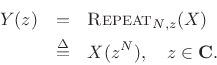
Downsampling (Decimation) Operator

**Figure:** Downsampling by .
$\includegraphics{eps/downsample}$

Figure 11.3 shows the symbol for downsampling by the factor . The downsampler selects every th sample and discards the rest:

$\begin{eqnarray*} y(n) &=& \hbox{\sc Downsample}_{N,n}(x)\\ &\isdef & x(Nn), \quad n\in{\bf Z} \end{eqnarray*}$

In the frequency domain, we have

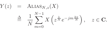
$\begin{eqnarray*} Y(z) &=& \hbox{\sc Alias}_{N,z}(X)\\ &\isdef & \frac{1}{N} \sum_{m=0}^{N-1} X\left(z^\frac{1}{N}e^{-jm\frac{2\pi}{N}} \right), \quad z\in{\bf C}. \end{eqnarray*}$

Thus, the frequency axis is expanded by the factor , wrapping times around the unit circle, adding to itself times. For , two partial spectra are summed, as indicated in Fig.11.4.

**Figure:** Illustration of **$\hbox {\sc Alias}_2$** in the frequency domain.
$\includegraphics[width=0.8\twidth]{eps/dnsampspec}$

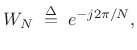
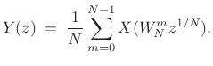
Using the common twiddle factor notation

$\displaystyle W_N \isdefs e^{-j2\pi/N},$

(12.1)

the aliasing expression can be written as

$\displaystyle Y(z) \eqsp \frac{1}{N} \sum_{m=0}^{N-1} X(W_N^m z^{1/N}).$

Example: Downsampling by 2

For , downsampling by 2 can be expressed as , so that (since $W_2\isdef e^{-j2\pi/2}=-1$ )

$\begin{eqnarray*} Y(z) &=& \frac{1}{2}\left[X\left(W^0_2 z^{1/2}\right) + X\left(W^1_2 z^{1/2}\right)\right] \\ [5pt] &=& \frac{1}{2}\left[X\left(e^{-j2\pi 0/2} z^{1/2}\right) + X\left(e^{-j2\pi 1/2}z^{1/2}\right)\right] \\ [5pt] &=& \frac{1}{2}\left[X\left(z^{1/2}\right) + X\left(-z^{1/2}\right)\right] \\ [5pt] &=& \frac{1}{2}\left[\hbox{\sc Stretch}_2(X) + \hbox{\sc Stretch}_2\left(\hbox{\sc Shift}_\pi(X)\right)\right]. \end{eqnarray*}$

Example: Upsampling by 2

For , upsampling (stretching) by 2 can be expressed as
$y=[x_0,0,x_1,0,\ldots]$ , so that

$\displaystyle Y(z) \eqsp X(z^2) \eqsp \hbox{\sc Repeat}_2(X),$

(12.2)

as discussed more fully in §2.3.11.

Filtering and Downsampling

Because downsampling by causes aliasing of any frequencies in the original signal above $\vert\omega\vert > \pi/N$ , the input signal may need to be first lowpass-filtered to prevent this aliasing, as shown in Fig.11.5.

**Figure 11.5:** Lowpass filtering followed by downsampling.
$\includegraphics[width=2in]{eps/downsampledfilter}$

Suppose we implement such an anti-aliasing lowpass filter as an FIR filter of length $M\le N$ with cut-off frequency $\pi/N$ .^12.1 This is drawn in direct form in Fig.11.6.

**Figure 11.6:** Direct-form implementation of an FIR anti-aliasing lowpass filter followed by a downsampler.
$\includegraphics[width=0.6\twidth]{eps/down_FIR}$

**Figure 11.7:** FIR lowpass filter with downsampler commuted inside the direct-form filter.
$\includegraphics[width=0.6\twidth]{eps/down_FIR_com}$

We do not need out of every filter output samples due to the : downsampler. To realize this savings, we can commute the downsampler through the adders inside the FIR filter to obtain the result shown in Fig.11.7. The multipliers are now running at times the sampling frequency of the input signal . This reduces the computation requirements by a factor of . The downsampler outputs in Fig.11.7 are called polyphase signals. The overall system is a summed polyphase filter bank in which each ``subphase filter'' is a constant scale factor . As we will see, more general subphase filters can be used to implement time-domain aliasing as needed for Portnoff windows (§9.7).

We may describe the polyphase processing in the anti-aliasing filter of Fig.11.7 as follows:

Subphase signal 0

$\displaystyle x(nN)\left\vert _{n=0}^{\infty}\right. \eqsp [x_0,x_N,x_{2N},\ldots]$ (12.3)

is scaled by .
Subphase signal 1

$\displaystyle x(nN-1)\left\vert _{n=0}^{\infty}\right.\eqsp [x_{-1},x_{N-1},x_{2N-1},\ldots]$ (12.4)

is scaled by ,
$\cdots$
Subphase signal

$\displaystyle x(nN-m)\left\vert _{n=0}^{\infty}\right.\eqsp [x_{-m},x_{N-m},x_{2N-m},\ldots]$

is scaled by .

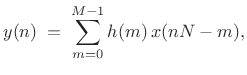These scaled subphase signals are finally summed to form the output signal shown in Fig.11.7

$\displaystyle y(n) \eqsp \sum_{m=0}^{M-1} h(m)\, x(nN-m),$

(12.5)

which we recognize as a direct-form-convolution implementation of a length FIR filter , with its output downsampled by the factor .

The summed polyphase signals of Fig.11.7 can be interpreted as ``serial to parallel conversion'' from an ``interleaved'' stream of scalar samples to a ``deinterleaved'' sequence of buffers (each length ) every samples, followed by an inner product of each buffer with $h = [h(0),\ldots,h(M-1)]$ . The same operation may be visualized as a deinterleaving through variable gains into a running sum, as shown in Fig.11.8.