Modeling a Continuous-Time System with Matlab

• Matlab
• Tutorials

Many of us are familiar with modeling a continuous-time system in the frequency domain using its transfer function H(s) or H(jω).  However, finding the time response can be challenging, and traditionally involves finding the inverse Laplace transform of H(s).  An alternative way to get both time and frequency responses is to transform H(s) to a discrete-time system H(z) using the impulse-invariant transform [1,2].  This method provides an exact match to the continuous-time impulse response.  Let’s look at how to use the Matlab function impinvar [3] to find H(z).   

This article is available in PDF format for easy printing.

Consider a 3^rd-order transfer function in s:

$$H(s)=\frac{c_3 s^3 + c_2 s^2 + c_1 s + c_0} {d_3 s^3 + d_2 s^2 + d_1 s + d_0 }$$

We want to transform it into a 3^rd order function in z:

$$H(z)=\frac{b_0 + b_1 z^{-1} + b_2 z^{-2} +b_3 z^{-3} } {1 + a_1 z^{-1} + a_2 z^{-2} + a_3 z^{-3} }$$

Which has a time response:

$$y_n = b_0 x_n + b_1 x_{n-1} + b_2 x_{n-2} + b_3 x_{n-3} - a_1 y_{n-1} -a_2 y_{n-2} -a_3 y_{n-3} $$

Given coefficients [c₃ c₂ c₁ c₀] and [d₃ d₂ d₁ d₀] of H(s), the function impinvar computes the coefficients [b₀ b₁ b₂ b₃] and [1 a₁ a₂ a₃] of H(z).

Example

A 3^rd order Butterworth filter with a -3 dB frequency of 1 rad/s has the transfer function [4,5]

$$H(s)=\frac{1} { s^3 + 2 s^2 + 2 s + 1 } \quad{(1)}$$

Here is the code to calculate the coefficients of H(z) using impinvar:

fs= 4;            % Hz
% 3rd order butterworth polynomial
num= 1;
den= [1 2 2 1];
[b,a]= impinvar(num,den,fs)     % coeffs of H(z)

b =    0.0000    0.0066    0.0056
a =    1.0000   -2.5026    2.1213   -0.6065

$$H(z)=\frac{.0066 z^{-1} + .0056 z^{-2} } {1 -2.5026 z^{-1} +2.1213 z^{-2} -.6065 z^{-3} }$$

Note we could also use b= [.0066 .0056], making the numerator .0066 + .0056z^-1, which would have the effect of advancing the time response by one sample. 

Now we can use the Matlab filter function to calculate the impulse response (Figure 1):

Ts= 1/fs;
N= 64;
n= 0:N-1;
t= n*Ts;
x= [1, zeros(1,N-1)];       % impulse
x= fs*x;                 % make impulse response amplitude independent of fs
y= filter(b,a,x);
plot(t,y,'.'),grid
xlabel('seconds')

Let’s compare this discrete-time response to the exact impulse response from the inverse Laplace Transform.  The inverse Laplace Transform of H(s) in equation 1 is [6]:

$$h(t)=[e^{-t} - \frac{2}{\sqrt{3}}e^{-t/2}cos(\frac{\sqrt{3}}{2}t + \frac{\pi}{6} )]u(t)$$

Figure 2 plots both responses -- the discrete-time result matches the continuous-time result exactly.

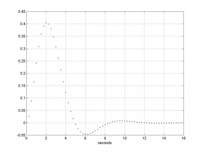
 Figure 1.  Impulse Response of discrete-time 3^rd order Butterworth Filter

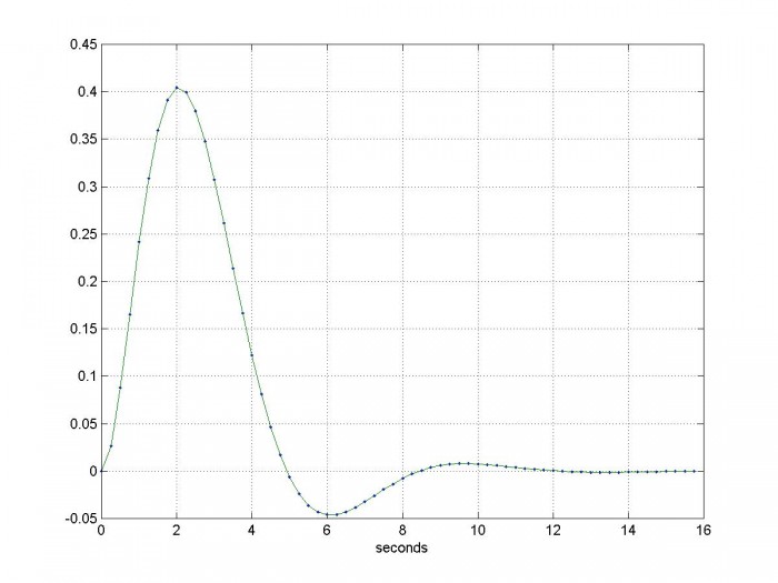
Figure 2.  Impulse Response   blue dots = discrete-time filter response

                        green = continuous-time filter response

We can also look at the step response:

x= ones(1,N);           % step
y= filter(b,a,x);       % filter the step

The continuous-time step response is given by [6]:

$$h(t)=[1 - e^{-t} - \frac{2}{\sqrt{3}}e^{-t/2}sin(\frac{\sqrt{3}}{2}t )]u(t)$$

Figure 3 plots both responses.  I had to advance the continuous-time response by T_s/2 to align it with the discrete-time response.  The responses don’t exactly match, but are very close – the error is plotted in figure 4.  The maximum error is only .0008.

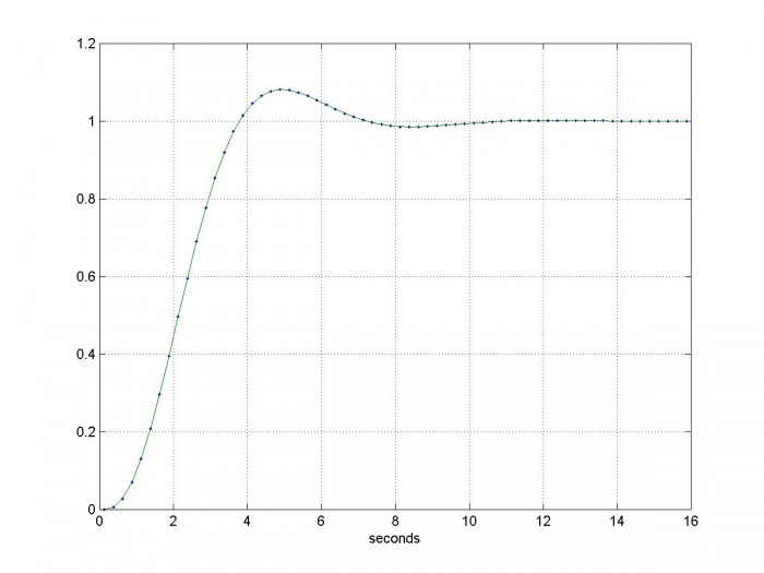
Figure 3.  Step Response 

blue dots = discrete-time filter response

               green = continuous-time filter response

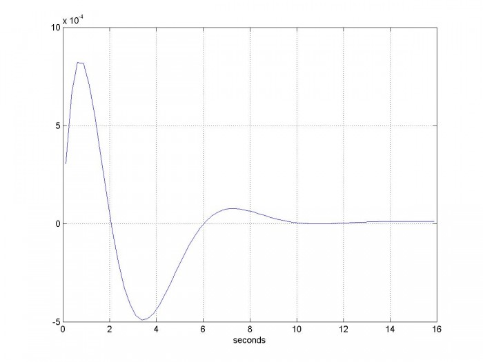
Figure 4.  Error of discrete-time step response

Now let’s look at the frequency response, and compare it to the continuous-time frequency response.  We use Matlab function freqz for the discrete-time frequency response, and freqs for the continuous-time frequency response:

[h,f]= freqz(b,a,256,fs);     % discrete-time freq response
H= 20*log10(abs(h));
w= 2*pi*f;
[hcont,f]= freqs(num,den,w);     % continuous-time freq response
Hcont= 20*log10(abs(hcont));
plot(w,H,w,Hcont),grid
xlabel('rad/s'),ylabel('dB')
axis([0 pi*fs, -80 10])

The results are plotted in Figure 5.  The discrete-time response begins to depart from the continuous-time response at roughly f_s/4.  To extend the accurate frequency range, we would need to increase the sample rate. 

Why use the discrete-time frequency response?  When modeling mixed analog/dsp systems, using the discrete-time response allows a single discrete-time model to represent the entire system.  You just need to be aware of the valid frequency range of the model.

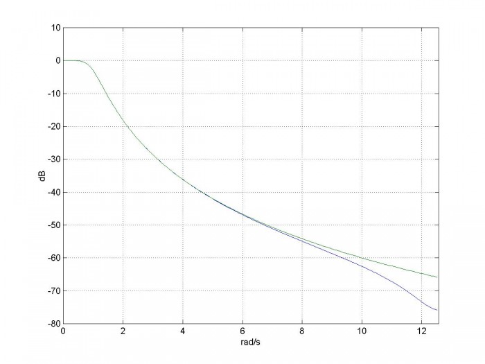
Figure 5.  Discrete-time (blue) and continuous-time (green) frequency responses

                   note: f_s/2 = 2 Hz = 12.57 rad/s

We can compute the group delay of the filter using the Matlab function grpdelay:

[gd,f]= grpdelay(b,a,256,fs);    % samples  Group Delay
D= gd/fs;                  % s  Group Delay in seconds
subplot(211),plot(w,H),grid
ylabel('dB')
axis([0 5 -50 10])
subplot(212),plot(w,D),grid
axis([0 5, 0 3])

The frequency response and group delay are plotted in Figure 6.  Note the group delay at 0 rad/s is 2 seconds.  This is equal to the delay of the peak of the impulse response in Figure 1.

Finally, note that the impulse-invariant transform is not appropriate for high-pass responses, because of aliasing errors.  To deal with this, a discrete-time low-pass filter could be added in cascade with the high-pass system to be modeled.   Or we could use the bilinear transform – see Matlab function bilinear [7].

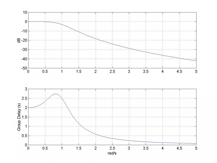
Figure 6.  Frequency Response and Group Delay of the discrete-time filter.

References

1.  Oppenheim, Alan V. and Shafer, Ronald W., Discrete-Time Signal Processing, Prentice Hall, 1989, section 7.1.1

2.  Lyons, Richard G., Understanding Digital Signal Processing, 2^nd Ed., Pearson, 2004, section 6.4

3.  https://www.mathworks.com/help/signal/ref/impinvar.html

4.  http://ecee.colorado.edu/~mathys/ecen2420/pdf/UsingFilterTables.pdf, p. 2

5.  Blinchikoff, Herman J. and Zverev, Anatol I., Filtering in the Time and Frequency Domains , Wiley, p. 110.

6.  Blinchikoff and Zverev, p. 116.

7.  https://www.mathworks.com/help/signal/ref/bilinear.html

% butter_3rd_order.m      6/4/17 nr
% Starting with the butterworth transfer function in s,
% Create discrete-time filter using the impulse invariance xform and compare
% its time and frequency responses to those of the continuous time filter.
% Filter fc = 1 rad/s = 0.159 Hz
% I.  Given H(s), find H(z) using the impulse-invariant transform
fs= 4;            % Hz  sample frequency
% 3rd order butterworth polynomial
num= 1;
den= [1 2 2 1];
[b,a]= impinvar(num,den,fs)         % coeffs of H(z)
%[b,a]= bilinear(num,den,fs)       
% II.  Impulse Response and Step Response
% find discrete-time impulse response
Ts= 1/fs;
N= 16*fs;
n= 0:N-1;
t= n*Ts;
x= [1, zeros(1,N-1)];   % impulse
x= fs*x;              % make impulse response amplitude independent of fs
y= filter(b,a,x);    % filter the impulse         
plot(t,y,'.'),grid
xlabel('seconds'),figure
% Continuous-time Impulse response from inverse Laplace transform
% Blinchikoff and Zverev, p116
h= exp(-t) - 2/sqrt(3)*exp(-t/2).*cos(sqrt(3)/2*t + pi/6); 
<p>e= h-y;                    % error of discrete-time response
plot(t,y,'.',t,h),grid
xlabel('seconds'),figure
% find discrete-time step response
x= ones(1,N);         % step
y= filter(b,a,x);    % filter the step         
% Continuous-time step response. Blinchikoff and Zverev, p116
t= t+Ts/2;                 % offset t to to align step responses
h= 1 - exp(-t) - 2/sqrt(3)*exp(-t/2).*sin(sqrt(3)/2*t); 
plot(t,y,'.',t,h),grid
xlabel('seconds'),figure
% III.  Frequency Response and Group Delay
% Find discrete-time and continuous time frequency responses
[h,f]= freqz(b,a,256,fs);     % discrete-time freq response
H= 20*log10(abs(h));
w= 2*pi*f;
[hcont,f]= freqs(num,den,w);     % continuous-time freq response
Hcont= 20*log10(abs(hcont));
plot(w,H,w,Hcont),grid
xlabel('rad/s'),ylabel('dB')
axis([0 pi*fs, -80 10]),figure
% Find group delay
[gd,f]= grpdelay(b,a,256,fs);   % samples  Group Delay
D= gd/fs;                  % s  Group Delay in seconds
subplot(211),plot(w,H),grid
ylabel('dB')
axis([0 5 -50 10])
subplot(212),plot(w,D),grid
axis([0 5, 0 3])
xlabel('rad/s'),ylabel('Group Delay (s)')

Neil Robertson    June, 2017

Sign in