The Discrete Fourier Transform as a Frequency Response

• DFT_FFT
• Tutorials

The discrete frequency response H(k) of a Finite Impulse Response (FIR) filter is the Discrete Fourier Transform (DFT) of its impulse response h(n) [1].  So, if we can find H(k) by whatever method, it should be identical to the DFT of h(n).  In this article, we’ll find H(k) by using complex exponentials, and we’ll see that it is indeed identical to the DFT of h(n).

Consider the four-tap FIR filter in Figure 1, where each block labeled T_s represents a delay of one sample time.  The filter has coefficients:

$$ h(n) = [h(0)\; h(1)\; h(2)\; h(3)]\qquad (1) $$

Note FIR coefficients are usually referred to as b(n).  We’re using the symbol h(n) to emphasize that the coefficients are equivalent to the filter’s impulse response.  We’ll find the frequency response of this filter, but first we need to derive the frequency response of the unit delay.

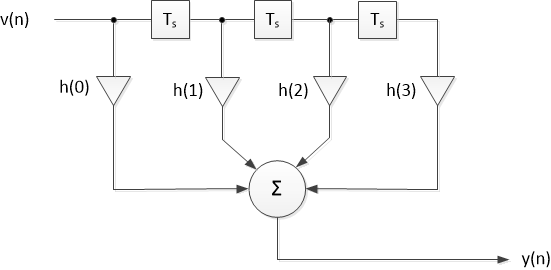
Figure 1.  FIR filter with four taps.

Frequency Response of the Unit Delay

Figure 2 shows a discrete-time unit delay of T_s, where T_s is the sample time.  In other words, this is a parallel data register clocked at f_s = 1/T_s.  Let the input be a discrete-time sinusoid of frequency f, with t = nT_s:

$$ v(n)= Acos(2\pi fnT_s) \qquad (2) $$

Now define a normalized radian frequency ω:

$$ \omega (rad) = 2\pi f/f_s = 2\pi f T_s \qquad (3) $$

This gives us:

$$ v(n)= Acos(n\omega) \qquad (4) $$

Then the output signal is:

$$ y(n)= Acos(2\pi f(nT_s - T_s)) = Acos(n\omega - \omega) \qquad (5) $$

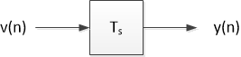
Figure 2.  Unit delay of a discrete-time signal.

Writing v and y as complex exponentials, we have:

$$ \mathbf{v}= Ae^{jn\omega} \qquad (6)$$

$$ \mathbf{y}= Ae^{j(n\omega - \omega)} = Ae^{jn\omega}e^{-j\omega} \qquad (7)$$

Given these expressions for v and y, the frequency response of the unit delay is simply:

$$ H_{UD}(\omega)= \frac{ \mathbf{y} }{\mathbf{v}} = e^{-j\omega} \qquad(8) $$

Frequency Response of the FIR Filter

We can now draw a frequency-domain model of the FIR filter (Figure 3), where the unit delays of Figure 1 have been replaced with H_UD = e^-jω.  Noting that e^-jω x e^-jω = e^-j2ω, we use Figure 3 to write the frequency response as:

$$ H(\omega)= \frac{Y(\omega)}{V(\omega)} = h(0)+h(1)e^{-j\omega}+h(2)e^{-j2\omega}+h(3)e^{-j3\omega} \qquad (9) $$

To be more general, if we let the FIR filter have any number of taps up to N, we can write:

$$ H(\omega)= \sum_{n=0}^{N-1} h(n)e^{-jn\omega} \qquad (10) $$

The normalized radian frequency ω is a continuous variable.  Let’s define a discrete f:

$$ f= \frac{kf_s}{N} \; ,k = 0: N-1 \qquad (11) $$

where k is the frequency index and N is the number of frequency samples (We have chosen to use the same number of frequency samples as filter coefficients).  Then, from Equation 3, discrete ω is:

$$ \omega= \frac{2\pi k}{N} \qquad (12) $$

Substituting this expression for discrete ω into Equation 10, we get:

$$ H(k)= \sum_{n=0}^{N-1} h(n)e^{-j2\pi kn/N} \qquad (13) $$

Equation 13 is a discrete-frequency version of the FIR frequency response of Equation 10.  But if you compare it to a textbook definition of the DFT [2, 3], you’ll see that Equation 13 is also the DFT of h(n)!  Thus we can write:

$$ h(n) \iff H(k) \qquad (14) $$

where the bi-directional arrow represents the DFT and inverse DFT.

In our derivation, we put no constraints on h(n), except that it contain no more than N samples.  So, we can substitute any discrete-time signal for h(n) in Equation 13, for example:

$$ X(k)= \sum_{n=0}^{N-1} x(n)e^{-j2\pi kn/N} \qquad (15) $$

Which is the DFT of the signal x(n).

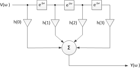
Figure 3.  FIR filter frequency-domain model.

Example

Given a 5-tap FIR filter with coefficients h = [1 2 3 2 1]/9, we can use Matlab and Equation 10 to find the magnitude of H(ω).  (Note we could also use Equation 13).  We’ll let N = 64, and we’ll compute ω using Equation 12:  ω =2πk/N.  Here is the Matlab code to compute H(ω):

    h0= 1/9; h1= 2/9; h2= 3/9; h3= 2/9; h4= 1/9;    % coeffs h(n)
    N= 64;                                        % number points in freq response
    k= 0:N-1;                                     % frequency index
    w= 2*pi*k/N;                          % vector of normalized radian frequencies
    H= h0+ h1*exp(-j*w) + h2*exp(-j*2*w) + h3*exp(-j*3*w) + h4*exp(-j*4*w);
    Hmag= abs(H)                          % magnitude of H(w)

The frequency response H(ω) is complex.  The magnitude of H(ω) is plotted vs. ω in Figure 4, where we can see the symmetry of the frequency response with respect to ω = π (f = f_s/2).  Suppose f_s = 100 Hz.  To plot the magnitude of H(f) vs f, we compute f from Equation 11:

    fs= 100;                    % Hz sample frequency
    f= k*fs/N;                  % frequency vector

The resulting plot is shown in Figure 5.  Finally, a more compact and efficient way to compute H(k) replaces h0, h1,… h4 and H in the above code with:

    h= [1 2 3 2 1]/9;          % signal vector
    H= fft(h,N);               % Matlab FFT function

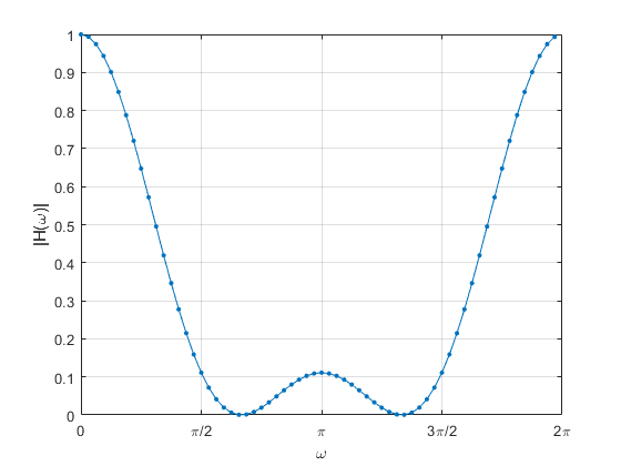
Figure 4.  Magnitude of H(ω), N = 64.

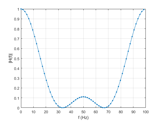
Figure 5.  Magnitude of H(f), N = 64, f_s = 100 Hz.

Conclusion

To review, we used complex exponentials to develop a formula for the continuous frequency response H(ω) (Equation 10) and discrete frequency response H(k) (Equation 13) of an FIR filter.  We then saw that the discrete frequency response is identical to the DFT of the filter’s impulse response h(n).  We also replaced h(n) in Equation 13 with x(n) to obtain the formula of the DFT of a general discrete-time signal (Equation 15).  You could say we used the FIR frequency response to develop the DFT formula.

A few topics not covered here:  To keep the math simple, I chose not to bring the z-transform into the discussion.  Also, since the FIR impulse response was inherently limited to N samples, there was no need to discuss spectral leakage or windowing.  I covered those topics in an earlier post [4].  Finally, the example computed the magnitude response of an FIR filter, but did not consider the phase response.  See [5] for a discussion of the phase response.

References

1.  Lyons, Richard, Understanding Digital Signal Processing, 3^rd Ed., Prentice Hall, 2011, p 179 – 180.

2.  Mitra, Sanjit K., Digital Signal Processing, 2^nd Ed., McGraw Hill, 2001, p 131.

3.  Lyons, p 60.

4.  Robertson, Neil, “The Discrete Fourier Transform and the Need for Window Functions”,

     DSPRelated.com, Nov. 15, 2021, https://www.dsprelated.com/showarticle/1433.php

5.  Lyons, section 5.8.

Neil Robertson          February, 2023

Sign in