


Multiplierless Half-band Filters and Hilbert Transformers
This article provides coefficients of multiplierless Finite Impulse Response 7-tap, 11-tap, and 15-tap half-band filters and Hilbert Transformers. Since Hilbert transformer coefficients are simply related to half-band coefficients, multiplierless Hilbert transformers are easily derived from multiplierless half-bands. Image attenuation of the Hilbert transformers presented here is greater than 50 dB over a bandwidth of 0.16*fs for the 7-tap version, 0.24*fs for the 11-tap version, and 0.3*fs for the 15-tap version, where fs is sample frequency.
The coefficient values and properties of the filters are summarized at the end of the article. Note that I discussed basics of half-band filters and Hilbert transformers in earlier posts [1,2].
7-Tap Half-band Filter
Here is a set of coefficients for a 7-tap half-band filter:
    b_hb = [-1/28 0 2/7 1/2 2/7 0 -1/28]
         = [-1 0 8 14 8 0 -1]/28              (1)
The sum of b is 1, so this filter has gain of 1 at f = 0 Hz. For a fixed-point [3,4] multiplierless filter, we’ll need a denominator that is a power of two. We can obtain this by multiplying the coefficients by 28/32 = 7/8, giving:
    b_hb = [-1 0 8 14 8 0 -1]/32
         = [-1/32 0 1/4 7/16 1/4 0 -1/32]     (2)
The filter now has a gain of 7/8 at f = 0 Hz.The filter block diagram is shown in Figure 1. All coefficients except for the center tap b3 are simply signed bit-shifts, while b3 is the sum of two signed bit-shifts. We can compute the filter’s magnitude response using Matlab:
    fs= 1;                          % Hz sample frequency
    b_hb= [-1 0 8 14 8 0 -1]/32;    % filter coefficients
    [H,f]= freqz(b_hb,1,256,fs);
    HdB= 20*log10(abs(H));          % dB-magnitude response
The dB-magnitude response is plotted in Figure 2. As expected for a half-band filter, the response magnitude at fs/4 with respect to that at f = 0 is -6 dB. Given that there are only seven taps, performance is modest. We could obtain a dc gain close to 1.0 by placing a gain of 9/8 in cascade with the filter: overall gain at dc would then be 9/8*7/8 = 63/64.
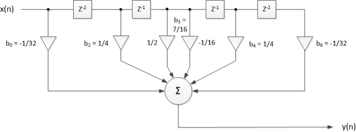
Figure 1. 7-tap Half-band filter block diagram. Blocks labeled z-2 represent a delay of 2 samples.
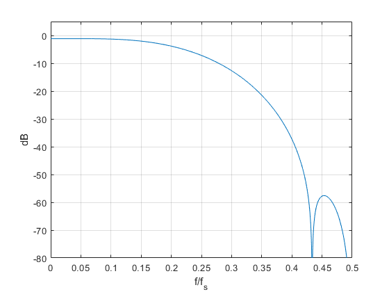
Figure 2. Magnitude response of 7-tap half-band filter. dc gain = 7/8.
7-Tap Hilbert Transformer
We learned about the relationship between the Hilbert Transformer and Half-band filter in an earlier post [5]. There, we found that Hilbert coefficients bHT(n) can be computed from a half-band design bHB(n) using the simple relationship:
$$b_{HT}(n)= 2 sin(n\pi /2)*b_{HB}(n),\quad -N/2 < n < N/2 \qquad (3) $$
where N is even and the number of taps is N + 1. For our 7-tap case, N = 6, n = -3: 3, and the value of sin(nπ/2) is:
sin(nπ/2) = [1 0 -1 0 1 0 -1] (4)
Given half-band coefficients of b_hb = [-1 0 8 14 8 0 -1]/32, Equation 3 results in Hilbert coefficients of:
b_ht = [b-3 0 b-1 0 b1 0 b3] = [-1 0 -8 0 8 0 1]/16 (5)
Note that bHT is odd-symmetric. All coefficients are realized with signed bit-shifts. The Hilbert transformer’s block diagram is shown in Figure 3, where we have re-numbered the coefficients to [b0 0 b2 0 b4 0 b6]. The half-band filter had a gain of 7/8 at f = 0, which causes the Hilbert transformer output xi to have a gain magnitude of 7/8 at f= fs/4. The center tap xr output must have the same gain as the xi output, so the center tap must be scaled by Gct = 7/8, as shown.
Now we’ll find the frequency response of the Hilbert Transformer. The transfer function H(z) is defined with respect to the center tap:
$$ H(z)= \frac{H_{FIR}(z)}{z^{-K}} \qquad (6) $$
Where HFIR(z) is the causal transfer function of the Hilbert transformer and K samples is the delay of the center tap. We can compute the frequency response of the Hilbert transformer using the following Matlab code:
    b= [-1 0 -8 0 8 0 1]/16;            % HT coefficients
    d= [0 0 0 1 0 0 0];                 % center tap = z^-3
    [H,f]= freqz(b,d,256,'whole',fs);   % freq. response over 0 to fs
Since the coefficients are odd-symmetric with respect to the center tap, the frequency response is pure imaginary, as shown in Figure 4. As expected, the gain magnitude at f = fs/4 is 7/8 = 0.875. The overall gain can be made close to 1.0 by placing a gain of 9/8 in cascade with the Hilbert transformer. If we choose to place the gain of 9/8 in cascade with the xr and xi outputs, a simplification in the xr path is possible: we can replace Gct with 9/8*Gct = 63/64 = 1 – 1/64.
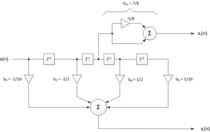
Figure 3. 7-tap Hilbert Transformer Block Diagram. Blocks labeled z-2 represent a delay of 2 samples.
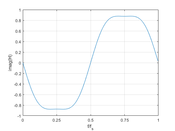
Figure 4. Pure-imaginary frequency response of 7-tap Hilbert transformer, Gct = 7/8 = 0.875.
7-tap Hilbert Transformer Image Attenuation
We have calculated the Hilbert transformer’s frequency response H(f), but this does not tell us anything about image attenuation. Let’s take a look at how to compute the image attenuation. Figure 5a shows a frequency-domain block diagram of a Hilbert Transformer. Its complex output spectrum is:
$$ X_c= X_r+ jX_i \qquad (7) $$
The frequency response of the complex output is:
$$ G(\omega)= \frac{X_r + jX_i}{X_r} \qquad (8) $$
or,
$$ G(\omega)= 1 + jH(\omega) \qquad (9) $$
where ω = 2πf/fs is normalized radian frequency. For an ideal Hilbert transformer, H(ω) = -j for 0 < ω < π and H(ω) = j for π < ω < 2π [2]. Thus G(ω) for the ideal case is given by:
$$G(\omega) = 2, \quad 0 < \omega < \pi \qquad \quad $$
$$ \qquad \qquad 0, \quad \pi < \omega < 2\pi \qquad (10) $$
Note that G(ω) is pure real. G(ω) for the ideal Hilbert transformer is plotted in figure 5b. The image band of π < ω < 2π has a response of 0.
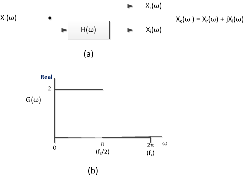
Figure 5. Hilbert transformer.
a) Frequency-domain block diagram. b) Frequency response of complex output for ideal case.
We can apply Equation 9 for our 7-tap transformer, but first we need to modify it to account for Gct used in Figure 3 and shown in Figure 6. G(ω) then becomes:
$$ G(\omega)= G_{ct} + jH(\omega) \qquad (11) $$
The magnitude of G(ω) at ω= π/2 (f = fs/4) is 2*Gct. We define a frequency response relative to this value as:
$$ G_{rel}(\omega) = \frac{G(\omega)}{2G_{ct}} \qquad (12) $$
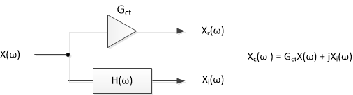
Figure 6. Hilbert Transformer frequency-domain block diagram for gain not equal to 1.0.
Now we’ll compute Grel(f), using Gct and H(f) that we found in the previous
section:
    Gct= 7/8;                % gain at f = fs/4
    G= Gct + j*H;            % freq. response of HT complex output
    Grel= G/(2*Gct);
    Grel_dB= 20*log10(abs(Grel));
Grel_dB is plotted in Figure 7. The image band is from 0.5*fs to fs. The red line in the image band shows the frequency range for 50 dB image attenuation. The corresponding passband centered at fs/4 is also shown: the bandwidth for 50 dB image attenuation is 0.16*fs. OK, not very wide bandwidth, but after all, we have only seven taps.
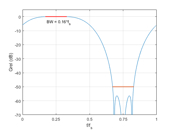
Figure 7. 7-tap Hilbert transformer. Frequency response Grel(f) of complex output, showing bandwidth for 50 dB image attenuation.
11-Tap Half-band Filter
Here is a set of coefficients for an 11-tap half-band filter:
    b_hb = [8 0 -40 0 192 319 192 0 -40 0 8]/1024
         = [1/128 0 -5/128 0 3/16 319/1024 3/16 0 -5/128 0 1/128]        (13)
These coefficients were synthesized as a Canonic Signed Digit (CSD) design. I discussed CSD filters in an earlier post [6]. The filter has gain of 639/1024 at f = 0. The coefficients can be realized as signed bit-shifts or sums of signed bit-shifts as indicated:
b0 = b10 = 1/128
b2 = b8 = -5/128 = -1/32 - 1/128
b4 = b6= 3/16 = 1/4 - 1/16 (or 1/8 + 1/16)
b5 = 319/1024 = 1/4 + 1/16 – 1/1024 (14)
The filter block diagram is shown in Figure 8, and the dB-magnitude response is plotted in Figure 9. The dc gain of 639/1024 causes the 4.1 dB insertion loss shown in the magnitude response. We could obtain a dc gain close to 1.0 by placing a gain of 3/2 in cascade with the filter: overall gain at dc would then be 1.5*639/1024 = 0.936.
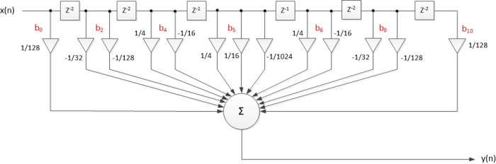
Figure 8. 11-tap half-band filter block diagram.
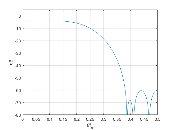
Figure 9. Magnitude response of 11-tap half-band filter. dc gain = 639/1024.
11-Tap Hilbert Transformer
Using Equation 3, we can derive a Hilbert transformer from the 11-tap half-band filter. The Hilbert transformer coefficients are:
    b_ht = [-1 0 -5 0 -24 0 24 0 5 0 1]/64
         = [-1/64 0 -5/64 0 -3/8 0 3/8 0 5/64 0 1/64]        (15)
As was the case for the half-band filter, the coefficients are sums of signed bit-shifts, as shown in Figure 10. The half-band filter had a gain of 639/1024 at f = 0, which causes the Hilbert transformer output xi to have a gain magnitude of 639/1024 at f= fs/4. The center tap xr output must have the same gain as the xi output, so the center tap must be scaled by Gct = 639/1024, as shown. The overall gain can be made close to 1.0 by placing a gain of 3/2 in cascade with the Hilbert transformer.
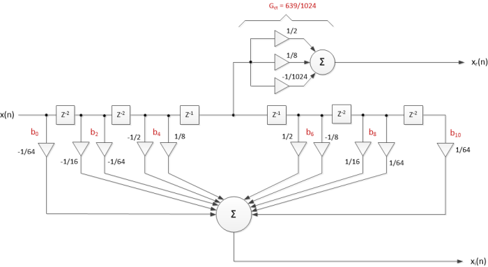
Figure 10. 11-tap Hilbert transformer block diagram.
The pure-imaginary frequency response of the Hilbert transformer is shown in Figure 11, where the gain magnitude at f = fs/4 is 639/1024 = 0.624. Grel_dB is plotted in Figure 7. The red line in the image band shows the frequency range for 50 dB image attenuation. The corresponding passband centered at fs/4 is also shown: the bandwidth for 50 dB image attenuation is 0.24*fs.
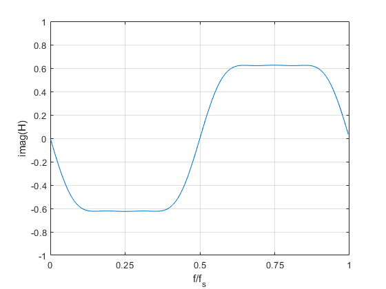
Figure 11. Pure-imaginary frequency response of 11-tap Hilbert transformer, Gct = 639/1024 = 0.624.
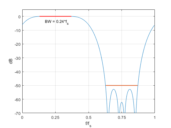
Figure 12. 11-tap Hilbert transformer. Frequency response Grel(f) of complex output, showing bandwidth for 50 dB image attenuation.
15-Tap Half-band Filter
Here is a set of coefficients for a 15-tap half-band filter:
b_hb = [-3 0 15 0 -48 0 194 316 194 0 -48 0 15 0 -3]/1024 (16)
As for the 11-tap case, these coefficients were synthesized as a CSD design. The filter has gain of 632/1024 at f = 0. The coefficients can be realized as sums of signed bit-shifts as indicated:
b0 = b14 = -3/1024 = -1/512 – 1/1024
b2 = b12 = 15/1024 = 1/64 – 1/1024
b4 = b10 = -48/1024 = -1/32 – 1/64
b6 = b8 = 194/1024 = 1/4 – 1/16 + 1/512
b7 = 316/1024 = 1/4 + 1/16 – 1/256 (17)
I have not included a block diagram of this filter. The filter’s dB-magnitude response is plotted in Figure 13, where we see that the dc gain of 632/1024 has caused an insertion loss of 4.2 dB. We could obtain a dc gain close to 1.0 by placing a gain of 3/2 in cascade with the filter: overall gain at dc would then be 1.5*632/1024 = 0.9258.
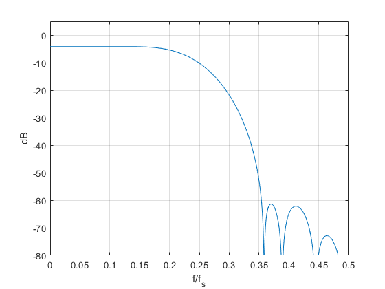
Figure 13. Magnitude response of 15-tap half-band filter. dc gain = 632/1024.
15-Tap Hilbert Transformer
Again using Equation 3, the 15-tap Hilbert transformer coefficients are derived from the 15-tap half-band coefficients as:
b_ht = [-3 0 -15 0 -48 0 -194 0 194 0 48 0 15 0 3]/512 (18)
These coefficients can be realized as sums of signed bit-shifts as indicated:
b0 = -b14 = -3/512 = -1/256 – 1/512
b2 = -b12 = -15/512 = -1/32 + 1/512
b4 = -b10 = -48/512 = -1/16 – 1/32
b6 = -b8 = -194/512 = -1/2 + 1/8 - 1/256 (19)
The half-band filter had a gain of 632/1024 at f = 0, which causes the Hilbert transformer output xi to have a gain magnitude of 632/1024 at f= fs/4. The center tap xr output must have the same gain as the xi output, so the center tap must be scaled by:
Gct = 632/1024 = 1/2 + 1/8 – 1/128 (20)
The overall gain can be made close to 1.0 by placing a gain of 3/2 in cascade with the Hilbert transformer.
The pure-imaginary frequency response of the Hilbert transformer is shown in Figure 14, where the gain magnitude at f = fs/4 is, as expected, 632/1024 = 0.6172. Grel_dB is plotted in Figure 15. The red line in the image band shows the frequency range for 50 dB image attenuation. The corresponding passband centered at fs/4 is also shown: the bandwidth for 50 dB image attenuation is 0.3*fs.
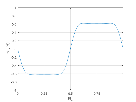
Figure 14. Pure-imaginary frequency response of 15-tap Hilbert transformer, Gct = 632/1024 = 0.6172
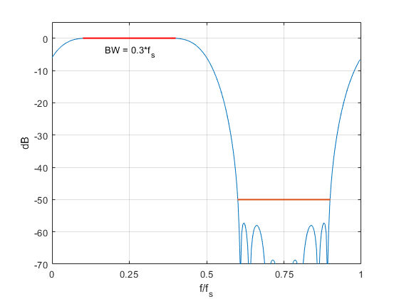
Figure 15. 15-tap Hilbert transformer. Frequency response Grel(f) of complex output, showing bandwidth for 50 dB image attenuation.
Summary
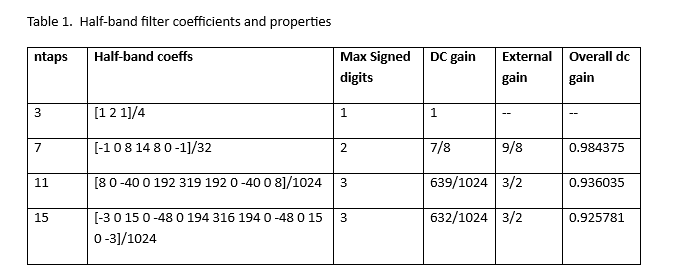
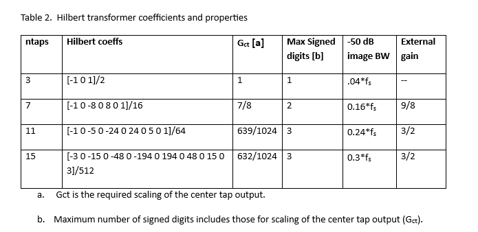
Tables 1 and 2 summarize the coefficients and properties of the filters we have discussed. All coefficients can be implemented as sums of (three or fewer) signed powers of 2, called “signed digits”. The tables include optional external gain for each filter to achieve an overall passband gain close to 1.0.
I have also included 3-tap versions of the half-band filter and Hilbert Transformer. The 3-tap half-band filter is identical to a linear interpolate-by-2 filter. The 3-tap Hilbert transformer’s coefficients are the negative of those of a central-difference differentiator.
References
1. Robertson, Neil, “Simplest Calculation of Half-band Filter Coefficients”, DSPrelated.com, Nov., 2017, https://www.dsprelated.com/showarticle/1113.php
2. Robertson, Neil, “Add the Hilbert Transformer to Your DSP Toolkit, Part 1”, DSPrelated.com, Nov, 2022, https://www.dsprelated.com/showarticle/1486.php
3. Felton, Christopher, “A Fixed-Point Introduction by Example”, DSPrelated.com, April, 2011, https://www.dsprelated.com/showarticle/139.php
4. Lyons, Richard, Understanding Digital Signal Processing, 3rd Ed., Pearson, 2011, section 12.1.
5. Robertson, Neil, “Add the Hilbert Transformer to Your DSP Toolkit, Part 2”, DSPrelated.com, Dec, 2022, https://www.dsprelated.com/showarticle/1487.php
6. Robertson, Neil, “Matlab Code to Synthesize Multiplierless FIR Filters”, DSPrelated.com, Oct, 2016, https://www.dsprelated.com/showarticle/1011.php
Neil Robertson October, 2023
- Comments
- Write a Comment Select to add a comment

Hi Neil.
It seems to me that your efficient half-band filters could be used as the initial decimation filters in a multistage decimation application, such as the following.
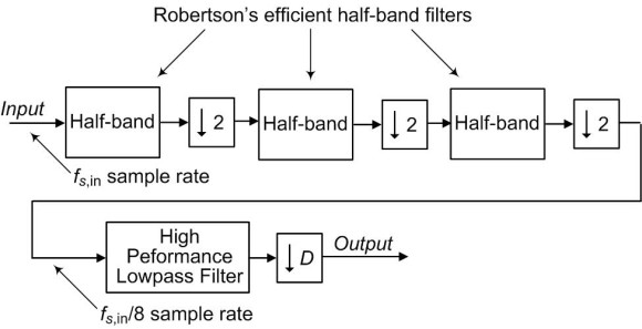
The advantage here is that the final traditional high-performance lowpass decimation filter is operating at the lowest sample rate. The coefficients of the final lowpass filter can be slightly increased in value to compensate for the slightly-less-than-unity gain of your efficient filters.

Hi Rick,
Thanks for suggesting this application, which is especially apt when the input sample rate is very high (e.g. 100's of MHz or GHz). The user should keep in mind that the stopband attenuation of these filters is on the order of 50 to 60 dB.
For this application, each half-band would have a different stopband frequency requirement, and the first half-band would require fewer taps than the 2nd half-band, which would require fewer taps than the 3rd half-band.
Neil

Hey Neil,
Nice work as always.
You should should pull all these together and show an example of a PLL locking to a phase/frequency reference. So that would be a delay/digital converter (or Hilbert transform), PLL design with multiplierlless feedback, and then using mu and enable to cross sample rate domains.
For the rest of the group these designs are tiny and can be implemented in a very small amount of fabric. Also way, way smaller and more power efficient if being done in an ASIC.
Cheers,
Mark Napier
Hi Mark,
I'm not sure I understand completely. Feel free to email me a block diagram.
regards,
Neil

Hi Neil,
Many thanks for your discussion. This one particularly took me far in the thinking.
Obviously your approach applies to any set of coeffs. The idea that you focused on is how to convert coeffs from multiplication requirement to shift. In doing so, obviously there was penalty of gain and limitations on the set itself and attenuation. It just occurred to me that filter design tools could have added such feature to their tool to target shift if preferred instead of try and see.
The other concept that popped up is that we also need to think of multiplications as repeated additions anyway but we may target less additions. I mean as an example, I can implement multiple additions for any coeff but that is what multiplication will do anyway. This gets questionable in FPGA that have dedicated mults (fabricated at silicone level) or it is done in the fabric (as adders) so doing adders is just equivalent to designing a mult in the fabric rather than targeting dedicated mults which may be a waste.
Your Hilbert filter response analysis puzzled me a lot. I have never done Hilbert filter. I had difficulty using freqz here as you did because my understanding is that the (a) in freqz(b,a) is 1 for FIR. I could be wrong.
So I then went to model the Hilbert filter as complex system with input of (real +j*0) outputting complex pair. But the filter is not doing internal complex multiplication. I mean when I enter freqz(b + j*a,1) it looks better but doesn't make sense as filter is not complex.
It is simpler for me to think of Hilbert as two separate branches: real part is just delayed while image part is a FIR so freqz(b,1) should be ok. What do you think?
Kaz,
Here is an alternative calculation of the Hilbert Transformer's frequency response. If you evaluate equation 6 with z= exp(jw), where w = 2*pi*k*fs/N, then the denominator is
denom = exp(-jwK)
here, lower case k is frequency index and uppercase K is delay of the HT center tap.
Here is the Matlab code to do this:
fs= 1;
N= 256;
k= 0:N-1; % frequency index
f= k*fs/N; % Hz frequency vector
w= 2*pi*f/fs; % rad norm rad freq.
b= [-1 0 -8 0 8 0 1]/16; % HT coefficients
K= 3; % samples delay of CT
Num= fft(b,N); % HT freq. response over 0 to fs
Den= exp(-j*w*K); % freq resp of CT
H= Num./Den;
To post reply to a comment, click on the 'reply' button attached to each comment. To post a new comment (not a reply to a comment) check out the 'Write a Comment' tab at the top of the comments.
Please login (on the right) if you already have an account on this platform.
Otherwise, please use this form to register (free) an join one of the largest online community for Electrical/Embedded/DSP/FPGA/ML engineers:


