Add the Hilbert Transformer to Your DSP Toolkit, Part 2

• Matlab
• Tutorials

In this part, I’ll show how to design a Hilbert Transformer using the coefficients of a half-band filter as a starting point, which turns out to be remarkably simple.  I’ll also show how a half-band filter can be synthesized using the Matlab function firpm, which employs the Parks-McClellan algorithm.

A half-band filter is a type of lowpass, even-symmetric FIR filter having an odd number of taps, with the even-numbered taps (except for the main tap) equal to zero.  This results in a frequency response with magnitude of 0.5 (-6 dB) at f = f_s/4.  In an earlier post [1], I derived the impulse response of an ideal half-band filter:

$$h_{HB}(n)= \frac{1}{n\pi} sin(n\pi /2), \qquad -\infty < n < \infty \qquad (1) $$

This impulse response, which is non-causal, is plotted in Figure 1 (top).  In Part 1 of this article, we saw (Equation 12) that the impulse response of an ideal discrete-time Hilbert Transformer is:

$$h_{HT}(n)= \frac{2}{n\pi} sin^2(n\pi /2), \qquad -\infty < n < \infty \qquad (2) $$

This impulse response is plotted in the bottom of Figure 1.  From these two equations we can write the Hilbert Transformer’s impulse response as:

$$h_{HT}(n)= 2sin(n\pi /2)*h_{HB}(n), \qquad -\infty < n < \infty \qquad (3) $$

Note that the sine values are {… 0, 1, 0, -1, 0 …}.  Equation 3 also applies for realizable half-band filters, as long as they are even symmetric, with the even-numbered taps equal to zero (except for the main tap).  We can write realizable Hilbert Transformer coefficients as:

$$b_{HT}(n)= 2sin(n\pi /2)*b_{HB}(n), \qquad -N/2 < n < N/2 \qquad (4) $$

where N is even and the number of taps is N + 1.  Our Hilbert Transformer design task has been reduced to design of a half-band filter.  Given that the sine values are {… 0, 1, 0, -1, 0 …}, we can see that, aside from the main tap, |b_HT(n)| = 2|b_HB(n)|.  

We note that multiplying the even-symmetric b_HB(n) by the odd-symmetric sine in Equation 4 results in b_HT(n) being odd symmetric with respect to the center tap.   b_HT(n) thus has a pure imaginary frequency response that is odd symmetric.  We can also view the Hilbert Transformer as a band-pass filter centered at f_s/4, that is realized by multiplying the half-band taps by a sine of frequency f_s/4:

$$b_{HT}(n)= 2sin[2\pi(f_s/4)nT_s]*b_{HB}(n)=2sin(n\pi /2)*b_{HB}(n), \quad -N/2 < n < N/2 \quad (5) $$

which agrees with Equation 4.

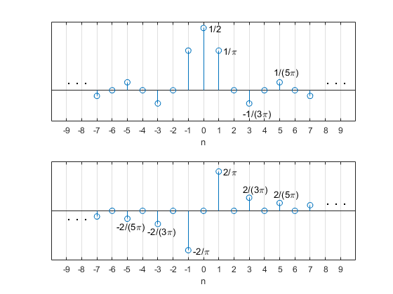
Figure 1.  Top: Ideal half-band filter impulse response.

                Bottom:  Ideal Hilbert Transformer impulse response.

Example 1.  Design of a 19-tap Hilbert Transformer

The appendix lists a short Matlab function hilbert_synth that uses Equation 4 to generate Hilbert Transformer coefficients from half-band filter coefficients.  In this example, we’ll use a 19-tap half-band filter (We’ll show how to calculate the half-band coefficients in Example 2).  The half-band coefficients and frequency response are plotted in Figures 2a and 2b.  The frequency response, which is pure real, was calculated relative to the center tap (as was done for a Hilbert Transformer in Part 1, Example 1).  The code to generate the Hilbert Transformer coefficients is as follows:

    % halfband filter coeffs
    b= [4 0 -21 0 64 0 -170 0 634 1024 634 0 -170 0 64 0 -21 0 4]/2048;
    b_hilb= hilbert_synth(b);
    b_hilb= round(b_hilb*1024)/1024;        % quantize coeffs

The quantized coefficients can be listed using:

b_hilb*1024

The calculated Hilbert Transformer coefficients are:

b_hilb = [-4 0 -21 0 -64 0 -170 0 -634  0  634 0 170 0 64 0 21 0 4]/1024.

The coefficients, which are the same as those used in the examples of Part 1, are plotted in Figure 2c.  Figure 2d plots the pure-imaginary frequency response, calculated relative to the center tap.  The passband of the frequency response is centered at f_s/4, as suggested by Equation 5.  The Hilbert Transformer’s image attenuation (defined in Part 1, Example 2) is plotted in Figure 3 using a dB amplitude scale.

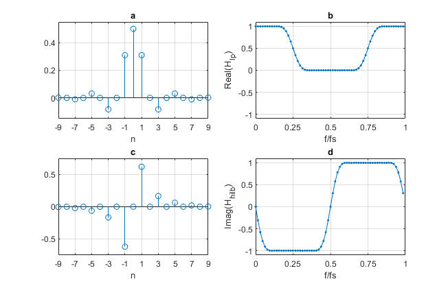
Figure 2.  19-tap Hilbert Transformer Synthesis from half-band filter.

a. Half-band coefficients.    b. Half-band filter frequency response relative to center tap.

c. Hilbert Transformer coefficients.    d. Hilbert frequency response relative to center tap.

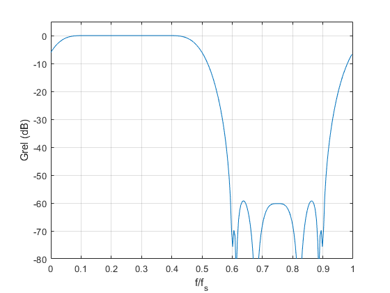
Figure 3.  19-Tap Hilbert Transformer image attenuation (see Part 1, Example 2).

Example 2.  Design of a 19-tap half-band filter using the Matlab function firpm

The half-band coefficients used in Example 1 were computed using the Matlab Parks-McClellan synthesis function firpm [2], as will now be described.  The function's inputs are filter order, a vector of passband and stopband frequency pairs, and an amplitude response goal vector.  The amplitude vs frequency goal for this example is plotted in Figure 4:  For f_s = 1, the passband edge is f_pass =0.15, and the stopband edge is 0.5 – f_pass.  For a half-band filter, the passband and stopband frequency ranges must be symmetrical with respect to fs/4.  The Matlab code to synthesize the filter is as follows:

    ntaps= 19;                    % number of taps
    N= ntaps-1;                   % filter order
    fpass= 0.15;                  % passband edge relative to fs
    f= [0 fpass .5-fpass .5]/.5;  % passband and stopband freq ranges
    a= [1 1 0 0];                 % amplitude response goal
    b= firpm(N,f,a);              % Parks-McClellan synthesis
    b= round(b*2048)/2048;        % quantize coeffs

Note that firpm uses frequencies relative to f_s/2, which requires dividing the frequency vector by 0.5.  The odd-symmetry of the response goal with respect to f_s/4 results in even-numbered taps (other than the main tap) being very close to zero.  They are then forced to zero by using rounding, as shown above.  The coefficients are the same as those listed at the beginning of Example 1:

b= [4 0 -21 0 64 0 -170 0 634 1024 634 0 -170 0 64 0 -21 0 4]/2048

The magnitude response is plotted in Figure 5, where we see that |H| is -6 dB at f_s/4.

A note on choosing half-band filter length:  Half-band filters must have an odd number of taps.  Also, for filters of length 5, 9, 13, …, the end coefficients are zero.  This means that the useful values of ntaps are 3, 7, 11, … That is, ntaps = 4K -1, K = 1,2,…  Filter order N is equal to ntaps – 1.

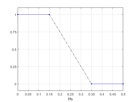
Figure 4.  Half-band filter response goal.  Passband = [0 0.15]; stopband = [0.35 0.5]

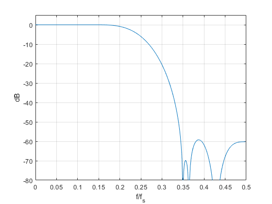
Figure 5.  Magnitude response of 19-tap half-band filter.  

Passband = [0 0.15]; stopband = [0.35 0.5]

Example 3.  Design of a 35-tap Hilbert Transformer

Here we again design a half-band filter and then compute Hilbert Transformer coefficients from the half-band coefficients.  The approach is the same as for Examples 1 and 2, but we change ntaps to 35 and increase the half-band passband edge fpass to 0.2.  We also decrease the coefficient quantization step from 1/1024 to 1/4096.

    % 1.halfband filter
    ntaps= 35;                      % number of taps
    N= ntaps-1;                     % filter order
    fpass= 0.2;                     % passband edge relative to fs
    f= [0 fpass .5-fpass .5]/.5;    % passband and stopband freq ranges
    a= [1 1 0 0];                   % amplitude response goal
    b_hb= firpm(N,f,a);             % Parks-McClellan synthesis
    % 2.find hilbert coeffs
    b_hilb= hilbert_synth(b_hb);
    b_hilb= round(b_hilb*4096)/4096;    % quantize coeffs
    b_hilb'*4096                        % list quantized coeffs

The resulting coefficients are:

b_hilb = [-9 0 -23 0 -47 0 -88 0 -152 0 -255 0 -431 0 -812 0 -2588   0   2588 0 812 0 431 0 255 0 152 0 88 0 47 0 23 0 9]/4096

The frequency response is plotted in Figure 6, along with that of the 19-tap version.  The image attenuation in dB is plotted in Figure 7, which shows markers at f/f_s = .05 and its image, f/f_s = .95.  The image level is about -63 dB.  So, this design provides greater than 60 dB image attenuation for frequencies as low as .05*f_s.  The frequency response in the passband is plotted in Figure 8.  The response is flat to within +/-.01 dB from .05*f_s to .45*f_s.

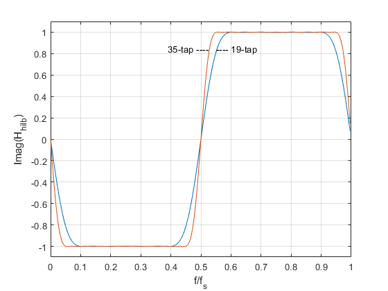
Figure 6.  35-tap and 19-tap Hilbert Transformer frequency responses.

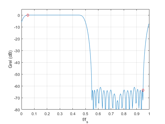
Figure 7.  35-tap Hilbert Transformer image attenuation.  Markers at f/f_s = .05 and 0.95

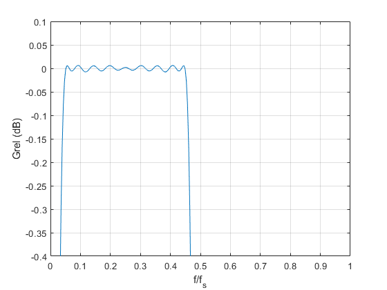
Figure 8.  35-tap Hilbert Transformer passband response (dB).

For the appendix, see the PDF version of this post.

References

1.  Robertson, Neil, “Simplest Calculation of Half-band Filter Coefficients”, DSPRelated, Nov. 20, 2017, https://www.dsprelated.com/showarticle/1113.php

2.  firpm, Matlab website, https://www.mathworks.com/help/signal/ref/firpm.html

Neil Robertson    December, 2022

Sign in