Weighted least-squares FIR with shared coefficients

• Matlab
• Design Methodolgies

FIR design with arbitrary routing between delay line and coefficient multipliers.

Includes a commented implementation of a generic IRLS FIR design algorithm.

Introduction: Reverse Engineering

While looking for numerical IIR filter optimization, a Matlab program in [1] for the design of FIR filters caught my attention. The equations looked familiar, sort of, but on closer examination the pieces refused to fit together.
Without the references, it took about two evenings to sort out how it works. And it worked in quite a different way than I had expected (maybe there is a lesson here, "don't assume anything...").
To my understanding, the algorithm is called "Lawson's method", or "iterative reweighted least-squares" (IRLS), and can be found in [2].

I ended up re-implementing it for complex-valued FIR coefficients, and used it to try an idea that had been on my mind for some time: FIRs with arbitrarily shared coefficients. That's what this blog is about, a feature not found in the usual design tools.
As there is no particular urgency to advertise the usefulness, value, importance etc. of this work, let me say this: the coefficient-sharing works as expected, but it's unlikely to be useful for typical design problems, as one cannot simply reuse a library component for the filter.

The second part continues with a discussion of the IRLS algorithm in general. I'll try to give a down-to-earth interpretation, since the code could be modified easily for other, non-standard FIR design problems.
The more mathematically-minded may continue reading in [1] page 19 (... uses Levinson's algorithm to solve the normal equations (2.9)).

Coefficient sharing FIRs

A FIR filter is the tool of choice in many communications applications, as it can achieve a constant group delay for all frequencies. For a filter running at high data rates, the implementation cost is mainly driven by the number of multiplications per sample. Avoiding multiplications can reduce hardware size and improve power consumption.

Special cases: symmetric and halfband FIR

The symmetric FIR filter is a well-known special case, as linear phase implies a symmetric impulse response if the absolute group delay is half the filter length. Pairs of delayed input samples share one coefficient, and about every second multiplier can be saved (Figure 1).

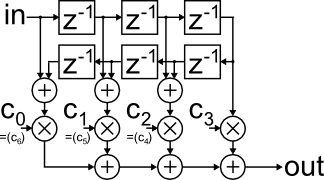
Figure 1: symmetric FIR implementation

As a side note, one could apparently get an additional tap "for free" by sharing also the final multiplier. Still, I chose an odd length, as reusing the last tap can cause more trouble than it's worth: The group delay of an even-length FIR falls halfway between two samples, and the FIR gets burdened with the additional, non-trivial task of implementing a half-sample delay.
Another implementation-friendly variant is the halfband filter, where every second coefficient is fixed to zero, at the price of a symmetric frequency response without independent control of pass- and stopband.

Arbitrary coefficient mapping

The idea of enforcing constraints between coefficients can be generalized to an arbitrary routing from delay taps to coefficients. For example, in a given filter, several taps may be "almost" equal, or some coefficients happen to be very close to zero. The motivation is that saving and reusing a multiplier allows a longer overall impulse response, which often has a considerable impact on performance.

Example

The frequency and impulse response in Figure 2 belong to a conventional, symmetric FIR filter with multiple stopbands. Note that the frequency response shows only the stopband area. The whole frequency range can be seen in Figure 8.
Opportunities for sharing coefficients are marked in the impulse response, where taps have almost identical values.

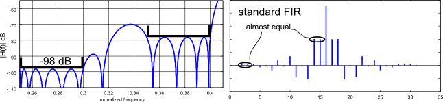
Figure 2: Frequency- and impulse response of conventional FIR filter

Now a FIR filter is to be designed that uses only one common coefficient for each pair of highlighted taps: The connections between coefficients and delay taps are given to the algorithm via a matrix such as the one shown in Figure 3: Columns correspond to delay taps, and rows to coefficients.
The circled entries route the near-equal taps from Figure 2 through one coefficient each. The letter "X" is used instead of 1 for better visibility.

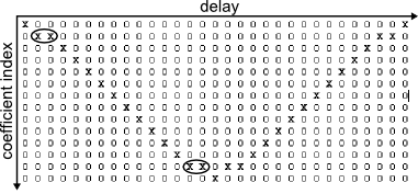
Figure 3: Coefficient routing matrix

The value of each matrix entry gives the relative weight of delay element x contributing through coefficient y. Non-equal weights could represent for example bit shifts (i.e. combine values with ratios of "almost" 2ⁿ).
Note, more systematic approaches to design for quantized coefficients exist, see for example [3].

The design algorithm then calculates a near-optimal filter for the constraints imposed by the coefficient routing (Figure 4):

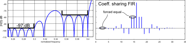
Figure 4: Frequency- and impulse response with shared coefficients

The coefficient-sharing leaves less freedom to the least-squares solver, so it is not surprising that stopband rejection degrades by 1.2 dB. Still, the filter achieves 97 dB, where a "conventional" FIR with two stages removed reaches only 92 dB (Figure 5):

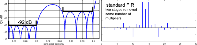
Figure 5: Conventional FIR with same number of multipliers as in Figure 4

The hand-tuned coefficient-sharing variant of the example filter achieves about 5 dB better performance than a conventional design that uses the same number of multipliers.
In a typical DSP application, saving two out of 16 multiplications does not justify the hassle and loss of flexibility. Nonetheless, the idea works and maybe it makes sense in high-speed or lowest-power applications, or on legacy hardware at the other end of the solar system.

IRLS algorithm

The ILRS algorithm designs the filter based on a nominal frequency response H(omega), an accuracy weighting factor, and (optionally) the coefficient routing matrix.

Design specification: [omega, H, w}

The usual requirements on a filter - passband gain/ripple and stopband attenuation - can be translated into a nominal frequency response H(f) and a tolerable deviation. Towards the design algorithm, H(f) appears as a linear quantity, in the same sense as sample magnitude, voltage or current (use 20 log₁₀|H(f)| to convert to dB).
For example, assuming a nominal passband gain of 0 dB and an allowed ripple of 0.5 dB, the magnitude error in |H(f)| is 6 percent: |H(f)| peaks at 1.06 instead of its nominal value 1.
The same error added to an ideal stopband would result in |H(f)| = 0.06 instead of 0, or -24.5 dB, . In order to be able to manipulate the frequency response at different frequencies (and for pass-/stopband individually), a weighting factor is introduced to scale the "importance" of an error at any frequency.
The concept is not completely straightforward, as the absolute pass-/stopband requirements are translated into relative weights. Details on calculating the weighting factor from requirements can be found here: Remez weights

The discussed algorithm is equally sensitive to amplitude- and phase error. However, the optimum (symmetric) FIR for a given magnitude response is linear-phase, and the remaining error is amplitude error only.

Iterative Reweighting loop

The "iterative reweighted least-squares" design algorithm consists of two distinct parts: An iterative reweighting outer loop, and a least-squares solver.
The reweighting loop is given a nominal frequency response and weighting factors. It sets up iteration weights from the weighting factors, hands them to the LS solver, and gets a FIR filter in return. It calculates the frequency response and determines the error to the nominal frequency response, weighs the error with the initial (!) weighting factors and adjusts the iteration weights, based on the outcome: Tighten, where the weighted error is large, relax where it is small.
The iteration weights are renormalized in each round, as only the ratio between frequencies matters, not the absolute value: It is obviously pointless to tell the LS solver "give me a better filter" - the LS solver would politely remind me that it is already least-squares optimal. Instead we should ask: "improve here and relax somewhere else".
Once the filter is designed, the cycle repeats: The updated iteration weights go back to the FIR solver, a new filter is returned, iteration weights are adjusted, etc. Iteration stops when the difference in the FIR coefficients between subsequent cycles falls below a threshold.

LS solver

The coefficients are determined by solving an equation system as shown in Figure 6. It states that the FIR filter with coefficients c transforms a sequence of input samples s into a sequence of output samples o. With one equation (matrix row) per coefficient, the solution is unique. So where is the "least-squares" part? As we'll see, all frequencies contribute to each row, thus resulting in a least-squares solution over all test frequencies.

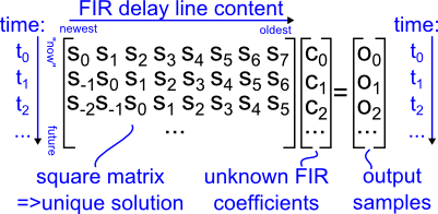
Figure 6: Equation system for FIR solver

Each matrix row can be interpreted as the state of samples in the FIR delay line, the first row at a time t₀, the second row at a time t₁ and so on. Each lower row results from time-shifting the upper row by one and feeding a fresh sample to the first position.

The indexing scheme of input samples may require some attention:
The most recent input sample at time t₀ has been named s₀, the next sample at time t₁ is s_-1, etc. This means, input samples with positive index have been fed into the delay line in the past, as they are already in place at time t₀ in the first matrix row.
Output sample o_i is generated at time t_i.

To summarize, matrix row y corresponds to time t_i, where the input and output sample to the FIR filter are s_-i and o_i, respectively. Note the minus sign! The reasons for the choice of indices will become clear later, in the context of Hermitian-Toeplitz matrix structure.

For the coefficient-sharing FIR, the time-delayed replicas of the input signal that are routed through any given coefficient are added in the matrix element that corresponds to the coefficient.

Construction of input and output samples

The input signal is constructed to result in a power spectrum that follows the iteration weights. This directs the LS-solver to be more accurate at some frequencies than at others. For a design with real-valued coefficients, the contribution at a single frequency omega_k is a cosine wave: cos(omega_kt) = real(exp(i omega_k t)). In the complex case, a rotating phasor exp(i omega_k t) is used. Either expression is scaled with the iteration weight for omega_k. In the output signal, the subexpression for each frequency is further scaled with the target frequency response H(omega), as the output signal is an ideal filter's response to the input signal. Time is not used explicitly, but a phase shift corresponding to one sample delay is repeatedly applied in the frequency domain.

LS solver example

Figure 7 illustrates, why the iterative reweighting-loop is needed: The least-squares solver alone tends to over-achieve where it is easy, but leaves too much error at the "difficult" corners.

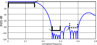
Figure 7: LS solver output for initial weights, no iterations

After iterating the weights, the following design results:

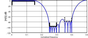
Figure 8: LS solver output after iterating the weights

Special case: Hermitian Toeplitz matrix structure

For a conventional FIR filter with one independent coefficient per tap, the matrix in Figure 6 has a Hermitian Toeplitz structure that allows use of the Levinson-Durbin algorithm to determine the FIR coefficients with reduced computational complexity(O(N ²) instead of O(N ³)). There are some implications to numerical accuracy, see [1] page 11 for a discussion.
Toeplitz implies that the signal is mirrored across the origin, and Hermitian that a conjugation takes place. In other words, each matrix entry must be the conjugate of its mirror image across the time axis. That is, s_x=conj(s _-x).
For a complex rotating phasor exp(i omega _k t), this is the case. The same applies to a real-valued cosine tone, since it can be rewritten as two complex phasors using 2 cos(a) = exp(i a)+exp(-i a). Only the first row of the matrix needs to be computed.

In the matlab implementation, coefficient-sharing FIRs result in a matrix that is not Toeplitz-structured, thus the equation system is built and solved by conventional means. I mention the concept here, as it was crucial to understanding the original code, and allows efficient filter design for an important special case. For an implementation, please refer to appendix B.1 in [1], program levin().

Matlab / Octave implementation (download)

The program can be downloaded here It should work on Matlab as well as Octave.

Latest version

A modified version of the algorithm can be downloaded here . It is not based on the normal functions of the least-squares problem, instead it uses weighted orthogonal signals for each frequency in the time domain. Also this program supports arbitrary coefficient routing, in particular symmetric FIR filters.

Summary

Coefficient sharing may shave off a multiplier or two in a FIR filter. Most likely, the benefits won't justify the effort for a run-of-the-mill design, but it may be useful in special applications, for example high-speed or low-power.
The included design program implements a generic IRLS algorithm that can be easily adapted for other non-standard FIR design problems (and of course, "standard" FIR design as well).

References

[1] Algorithms for the Constrained Design of Digital Filters with Arbitrary Magnitude and Phase Responses

[2] C. L. Lawson Contributions to the Theory of Linear Least Minimum Approximations Ph. D. dissertation, Univ. Calif., Los Angeles, 1961.

3 Design of low-complexity FIR filters based on signed powers-of-two coefficients with reusable common subexpressions

Sign in