Instantaneous Frequency Measurement

• Matlab
• FPGA
• Basics

I would like to talk about the oft used method of measuring the carrier frequency in the world of Signal Collection and Characterization world. It is an elegant technique because of its simplicity. But, of course, with simplicity, there come drawbacks (sometimes...especially with this one!).

In the world of Radar detection and characterization, one of the key characteristics of interest is the carrier frequency of the signal. If the radar is pulsed, you will have a very wide bandwidth, a short burst but great SNR. If on the other hand, it is a spread spectrum radar, you will have a signal that is present for a long time but the SNR is low and hence processing and extracting information becomes a challange. In the first case, we need a technique that is able to give us an answer on the center frequency with very little information available. In the second case, we need to have a technique that is resiliant enough to operate in degraded conditions. IFM is one such technique. I will talk about the drawbacks in just a little bit.

Let us look at the basic mathematical foundation real quick:

Let us start with a simple example of a simple sinusoid with a constant amplitude.

s(t) = Acos(ωt + Φ)

where A is the constant amplitude, ω is the angular frequency and Φ is the initial phase.

If we were to delay this signal by some τ and multiply it with the original signal we will have:

s(t)s(t+τ) = Acos(ωt + Φ)Acos(ω(t+τ)+Φ)

s(t)s(t+τ) = A²⁄2·[cos(2ωt+ωτ+2Φ) - cos(-ωτ)]

If we low pas filter the above delay multiplied signal, we are left with:

s1(t) = -A²⁄2·cos(ωτ)

Now, if we were to measure the signal s(t) and s(t+τ) we can have the experimental value s1(t). If we perform the angle calculation (inverse cosine), we will end up with

ω = [arccos(-2s1(t)/A²)-Φ + 2kπ]/τ

Thing to note in digital systems is that we would typically have an analytic signal for processing rather than a real signal. This makes the arccos into an arctan. Still an expensive operation on a FPGA! So in the digital case, the s[n] we would be looking at would be an imaginary signal. If we follow though with the math above given s[n] = Aexp[ωn+Φ], we would arrive at a similar formula for ω above except the arccos will be substituted by an arctan.

Thing to note as well is that in either case (original signal real or complex) there is this 2 pi ambiguity. This will make our signal alias over the 2-pi interval. Hence we need to find a way to resolve this ambiguity. This is easily done by the observation that if we pick multiple delays (τ) and have multiple delay-multiply values, we can find the exact frequency. This is demonstrated through the following figures. This was done in MATLAB and you might find the attached script useful.

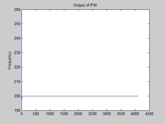
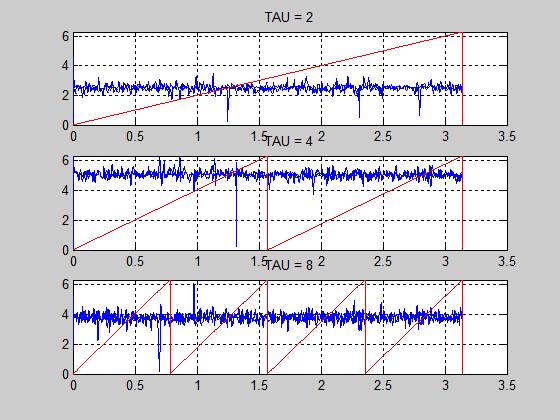
In the first two plots, the SNR is infinite. The sampling rate used is 1000 and the center frequency of the signal is 200. I have used three different delays (delay = 2, 4, 8). The plots of these delays are shown. Also shown is the output frequency of the IFM.

In the above plot, my intention with the arrows at the intersections is to show the ambiguity as τ increases. In short, while the resolution increases with τ, so does the ambiguity.

The graph of the frequency is:

Now, if we look at the phase and frequency output for the same signal with a SNR of 2dB over the full bandwidth, following are the results:

And frequency:

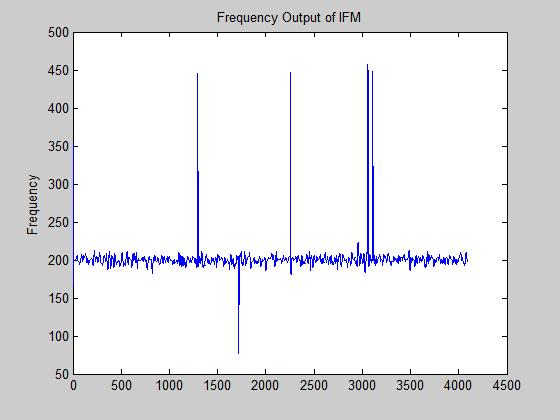
Some interesting features arise when the frequency we are trying to measure is related to the angles pi/4, pi/2, pi etc. because ωτ for various τ can give us a number that is either close to or exactly pi, 2pi, 0 etc. The issue with a number close to 0 or 2pi is the fact that the measured phase will jump between 0 and 2pi with noise. This will also ruin our frequency measurement. This is illustrated in the two figures below:

In the above two figures, the SNR is still 2dB but the frequency is now 240. The angular frequency for f = 240 is (240*2pi/1000). For delay of 4, ωτ ≈ 2pi. With noise, this value of ωτ will jump rapidly between 0 and 2pi as noticed in subplot 2 above. Also, for delay of 8, ωτ ≈ 4pi. Again, this value will jump between 0 and 2pi as shown in subplot 3 above. If you look at the frequency output now, it is quite noisy. A way to alleviate this problem is to unwrap the phase measurements.

The major drawback of the IFM scheme is presence of in band interferers. If the interferer is stronger than the signal we are trying to measure, the IFM will "pull" the result towards the stronger signal. In the digital realm, this is mitigated by having smaller bandwidths of interest and using channelizers.

The MATLAB code that I used to generate is as below:

fs = 1000;
fc = 240
t = 0:1/fs:4095/fs;
s = awgn(floor(127*cos(2*pi*fc*t)),2,'measured');
s_imag = hilbert(s);
d1 = 2;
d2 = 4;
d3 = 8;
lpf = [-2.6498e-019 7.977e-005 0.00036582 0.00095245 0.0019625 0.0035319 0.0057835 0.0087932 0.012558 0.01697 0.021811 0.026759 0.031423 0.035391 0.038282 0.039806 0.039806 0.038282 0.035391 0.031423 0.026759 0.021811 0.01697 0.012558 0.0087932 0.0057835 0.0035319 0.0019625 0.00095245 0.00036582 7.977e-005 -2.6498e-019];
s_d1 = [s_imag(d1+1:end) zeros(1,d1)];
s_d2 = [s_imag(d2+1:end) zeros(1,d2)];
s_d3 = [s_imag(d3+1:end) zeros(1,d3) ];

delay1 = angle(filter(lpf,1,s_d1.*conj(s_imag)));
delay2 = angle(filter(lpf,1,s_d2.*conj(s_imag)));
delay3 = angle(filter(lpf,1,s_d3.*conj(s_imag)));

delay1(delay1<=0) = delay1(delay1<=0) + 2*pi;
delay2(delay2<=0) = delay2(delay2<=0) + 2*pi;
delay3(delay3<=0) = delay3(delay3<=0) + 2*pi;

k1 = zeros(size(delay1));
k2 = zeros(size(delay2));

k1(delay1 > pi) = 2;
k2(delay2 > pi) = 1;

k = k1+k2;

w = (delay3 + 2*k*pi)/d3;
f = fs*w/(2*pi);

x = linspace(0,pi,size(delay3,2));
y1 = mod(2*x, 2*pi);
y2 = mod(4*x, 2*pi);
y3 = mod(8*x, 2*pi);
figure(1);
subplot(3,1,1); plot(x,delay1); hold on; plot(x, y1,'r'); title('TAU = 2'); grid on; set(gca, 'Ylim', [0 2*pi]);
subplot(3,1,2); plot(x,delay2); hold on; plot(x, y2,'r'); title('TAU = 4'); grid on; set(gca, 'Ylim', [0 2*pi]);
subplot(3,1,3); plot(x,delay3); hold on; plot(x, y3,'r'); title('TAU = 8'); grid on; set(gca, 'Ylim', [0 2*pi]);

figure(2);
plot(f); ylabel('Frequency'); title('Frequency Output of IFM')

You can play around with different sampling frequencies, center frequencies and SNRs to see how well the scheme works. You can also change the signal so that instead of being a simple sinusoid its a FM, phase coded or something else. I think, given the speed with which you arrive at an answer and relative implementation simplicity on a FPGA makes this scheme attractive.

I would like to add that please feel free to ask questions. If the concept of resolving the ambiguity is not clear, I can write up another short blog regarding how that works out. Hopefully you will be able to decipher the details from the MATLAB script. But if not, let me know.

References:

1. "Digital Techniques for Wideband Receivers" by James Tsui

Sign in