


Ten Little Algorithms, Part 2: The Single-Pole Low-Pass Filter
Other articles in this series:
- Part 1: Russian Peasant Multiplication
- Part 3: Welford's Method (And Friends)
- Part 4: Topological Sort
- Part 5: Quadratic Extremum Interpolation and Chandrupatla's Method
- Part 6: Green’s Theorem and Swept-Area Detection
I’m writing this article in a room with a bunch of other people talking, and while sometimes I wish they would just SHUT UP, it would be better if I could just filter everything out. Filtering is one of those things that comes up a lot in signal processing. It’s either ridiculously easy, or ridiculously difficult, depending on what it is that you’re trying to filter.
I’m going to show you a one-line algorithm that can help in those cases where it’s ridiculously easy. Interested?
Here’s a practical example of a filtering problem: you have a signal you care about, but it has some noise that snuck in through a little hole in the wall, and darnit, you’re stuck with the noise.
import matplotlib.pyplot as plt
import numpy as np
np.random.seed(123456789)   # repeatable results

f0 = 4
t = np.arange(0,1.0,1.0/65536)
mysignal = (np.mod(f0*t,1) < 0.5)*2.0-1
mynoise = 1.0*np.random.randn(*mysignal.shape)

plt.figure(figsize=(8,6))
plt.plot(t, mysignal+mynoise, 'gray',
         t, mysignal,         'black');
And the question is, can we get rid of the noise?
Here we’ve got a lot of noise: relative to a square-wave signal with peak-to-peak amplitude of 2.0, the peak-to-peak noise waveform is in the 6-7 range with even larger spikes. Yuck.
The signal processing approach is to look at the frequency spectrum.
def spectrum(x):
    return np.abs(np.fft.ifft(x))

mysignal_spectrum = spectrum(mysignal)
mynoise_spectrum  = spectrum(mynoise)
N1 = 500
f = np.arange(N1)
plt.figure(figsize=(8,4))
plt.plot(f,mysignal_spectrum[:N1])
plt.plot(mynoise_spectrum[:N1])
plt.xlim(0,N1)
plt.legend(('signal','noise'))
plt.xlabel('frequency')
plt.ylabel('amplitude')
Now this is some good news for signal processing. The signal spectrum content really stands out above the noise. Square waves have harmonics that are odd multiples of the fundamental frequency: here 4Hz, 12Hz, 20Hz, 28Hz, etc. The harmonic content decays as 1/f. White noise, on the other hand, has a roughly flat spectrum that is spread out across all harmonics, so it is lower in amplitude for the same amount of energy. Kind of like making a peanut butter sandwich — if you put a glob of peanut butter on a slice of bread, it’s pretty thick, but if you spread it over the bread evenly, it’s much thinner, even though it’s the same amount of peanut butter. Mmmm. I hope you like peanut butter; this is making me hungry.
This effect is easier to see on a log scale:
z0 = 1e-10  # darnit, we have to add a small number so log graphs don't barf on zero
for N1 in [500, 8000]:
    f = np.arange(N1)
    plt.figure(figsize=(8,4))
    plt.semilogy(f,z0+mysignal_spectrum[:N1],f,z0+mynoise_spectrum[:N1])
    plt.xlim(0,N1)
    plt.ylim(1e-4,1)
    plt.legend(('signal','noise'))
    plt.xlabel('frequency')
    plt.ylabel('amplitude')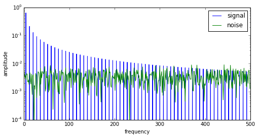
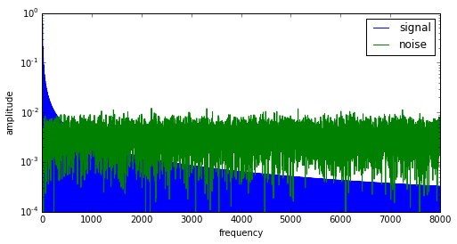
What we’d really like is to keep the low frequencies only; most of the signal energy is only in the lowest harmonics, and if we want to get rid of the noise, there’s no point in keeping the higher frequencies where the noise energy is much higher. Looks like the crossover here is roughly around 500Hz; below 500Hz the signal dominates, and above that point the noise dominates.
So let’s do it! We’ll use a low-pass filter to let the low frequencies pass through and block the high frequencies out.
In an ideal world, we’d use a low-pass filter with a very sharp cutoff, in other words one that lets everything through below 500Hz and nothing through above 500Hz. But in practice, sharp-cutoff filters are challenging to implement. It’s much easier to create a gradual-cutoff filter, and the simplest is a single-pole infinite impulse response (IIR) low-pass filter, sometimes called a exponential moving average filter.
We’re going to use a filter which has a transfer function of \( H(s) = \frac{1}{\tau s + 1} \). This is a first-order system, which I’ve talked about in a previous article, in case you’re interested in more information. But here we’re just going to use it.
We’ll start with the differential equation of this filter, which is \( \tau \frac{dy}{dt} + y = x \).
We can take this continuous-time equation and convert to a discrete-time system with timestep \( \Delta t \), namely \( \tau \frac{\Delta y}{\Delta t} + y = x \), and if we solve for \( \Delta y \) we get \( \Delta y = (x-y)\frac{\Delta t}{\tau} \). Blah blah blah, math math math, yippee skip. Here’s the upshot, if all you care about is some computer code that does something useful:
//
// SHORTEST USEFUL ALGORITHM ****EVER****
//

y += alpha * (x-y);

//
//    # # #   ##    ##   #####  #
//    # # #  #  #  #  #    #    #
//    # # #  #  #  #  #    #
//     # #    ##    ##     #    #
//
That’s it! One line of C code. The input is x. The output is y. The filter constant is alpha. Every timestep we add alpha times the difference between input and output. So simple.
Now we just have to calculate what alpha is. The approximate answer is \( \alpha = \frac{\Delta t}{\tau} \): we just divide \( \Delta t \) by the time constant \( \tau \). The more accurate answer is \( \alpha = 1 - e^{-\Delta t/\tau} \approx \frac{\Delta t}{\tau} \), with the approximation being more accurate for time constants much longer than the timestep, namely \( \tau \gg \Delta t \).
Let’s see it in action. If we want to have a filter with a cutoff of 500Hz (in other words, pass through frequencies much lower than 500Hz, block frequencies much higher than 500Hz), we use a value of \( \tau \) = 1/500 = 2msec.
def lpf(x, alpha, x0 = None):
    y = np.zeros_like(x)
    yk = x[0] if x0 is None else x0
    for k in xrange(len(y)):
        yk += alpha * (x[k]-yk)
        y[k] = yk
    return y

delta_t = t[1]-t[0]
tau = 0.002
alpha = delta_t / tau

plt.figure(figsize=(8,6))
y1 = lpf(mysignal+mynoise, alpha, x0=0)
plt.plot(t,y1)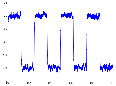
Hey, that’s not bad, especially considering that the original signal including noise had a huge amount of noise on it. There is always a tradeoff in filtering: if you want less noise, you can use a lower cutoff frequency, at the cost of more phase lag. Phase lag is a frequency-dependent delay that rounds off sharp edges and plays havoc with feedback control systems, if they aren’t designed to take that phase lag into account. We could use a lower cutoff frequency here, say 100Hz → \( \tau \) = 10 msec:
tau = 0.010
alpha = delta_t / tau

plt.figure(figsize=(8,6))
y2 = lpf(mysignal+mynoise, alpha, x0=0)
plt.plot(t,y2)
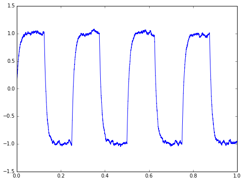
There you go: less noise, more rounding / distortion / phase lag / whatever you want to call it.
Here are the signal spectra for signals shown in the two previous graphs:
N1 = 500
f = np.arange(N1)
plt.figure(figsize=(8,4))
plt.semilogy(f,spectrum(y1)[:N1],'.',f,spectrum(y2)[:N1],'+')
plt.xlim(0,N1)
plt.ylim(1e-4,1)
plt.legend(('tau = 2msec','tau = 10msec'))
plt.xlabel('frequency')
plt.ylabel('amplitude')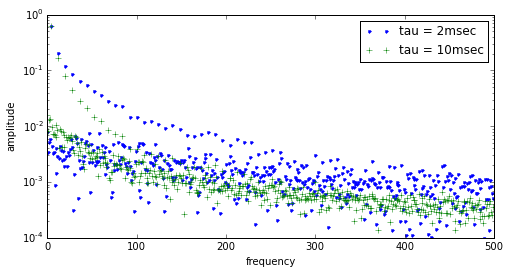
The higher time constant filter has a lower cutoff frequency, so the remaining amplitude of the output signal is lower.
Now in practice, this example we’ve used contains a huge amount of noise on the input signal. We always hope for signals that are less noisy than that. Here’s a more reasonable example, with only 10% of the noise we showed earlier:
mynoise2 = 0.1*np.random.randn(*mysignal.shape)
alpha=delta_t/0.0005
lpf_out2 = lpf(mysignal+mynoise2, alpha=alpha, x0=0)

fig=plt.figure(figsize=(8,10))
ax=fig.add_subplot(3,1,1)
ax.plot(t,mysignal+mynoise2,t,mysignal)
ax.set_ylabel('original signal')
ax2=fig.add_subplot(3,1,2)
ax2.plot(t,lpf_out2)
ax2.set_ylabel('lpf output')
ax3=fig.add_subplot(3,1,3)
ax3.plot(t,lpf_out2)
ax3.set_ylim(-1.05,-0.95)
ax3.set_ylabel('lpf output, zoom')
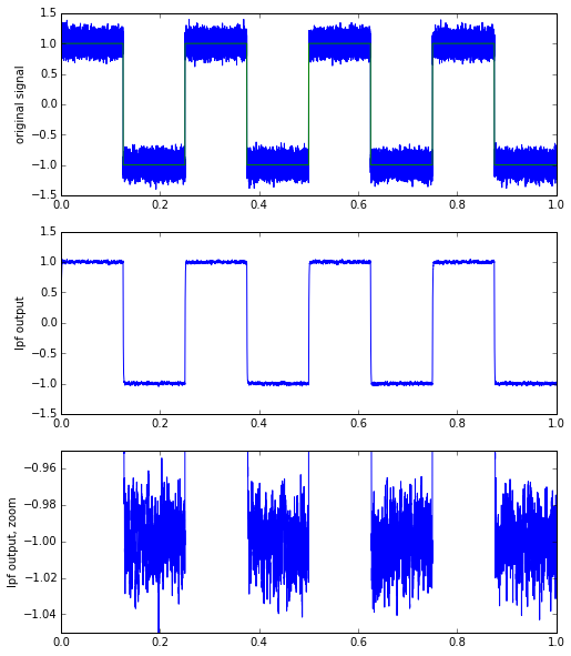
Here we can go all the way out to a cutoff frequency of 2000 Hz (time constant of 0.5 msec), get fairly nice edges in our signal, but still remove most of the noise. In general the noise content gets reduced in amplitude by a factor of about \( \sqrt{\alpha} \): here we have \( \alpha = \Delta t/\tau = 1.0/f\tau \) where f is the sampling frequency, and for f = 65536Hz we have \( \alpha = 1/32.768 \), so should expect about a reduction to about 1/5.7 of the original noise level. We might have had a peak-to-peak noise of about 0.5 in the original signal, and we’re down to maybe 0.08 now, which is around 1/6 of the original noise level. Measuring peak noise is kind of subjective, but we’re in the ballpark of what theory predicts.
The interesting thing here is the value \( \alpha \) drops if the timestep \( \Delta t \) gets smaller: we can improve the noise filtering if we sample more often. This is called oversampling and it can be used, up to a point, to reduce the impact of noise on signals of interest, by sampling them more than normal and then using low-pass filters to get rid of the noise. Oversampling has diminishing returns, because if we want half the noise amplitude, we have to sample four times as often, and compute the filter four times as often. It also only works on noise. If our unwanted signal is, say, a Rick Astley song, with the same general type of frequency spectrum content of our signal of interest, then we’re totally out of luck if we try to filter it out, and we just have to hope the person playing it has some sense of decency and will turn it off.
Fixed-point implementation of a low-pass filter
The one line of code posted above:
// curtains part, angels sing....

y += alpha * (x-y);

// now back to normal
is applicable for floating-point math. Most of the lower-end processors don’t have floating-point math, and have to emulate it, which takes time and CPU power. If you want to work in fixed-point instead, the code to implement a low-pass filter looks like this:
y_state += (alpha_scaled * (x-y)) >> (Q-N);
y = y_state >> N;
where alpha_scaled = \( 2^Q \alpha \) for some fixed-point scaling Q, and you have to keep N additional state bits around to accurately represent the behavior of the low-pass filter. The value of N is more or less logarithmic in alpha, e.g. \( N \approx - \log_2 \alpha \), so if you want to use very long time constants, you have to keep around more bits in your filter state. I worked with a software contractor around 2002 or 2003, who was convinced I was wrong about this; if I wanted to filter a 16-bit ADC reading, what was wrong about storing everything in 16 bits? Why would I have to use 32-bit numbers? But you do; try it without adding extra bits: you’ll find that there is a minimum difference in input that is needed in order to get the output to change, and small changes in the input will make the output look stair-steppy. This is an unwanted quantization effect.
Don’t believe me? Let’s try it, first with floating-point, then with fixed-point, on a pair of signals. Signal x1 will be a square wave plus some unwanted high-frequency stuff; signal x2 will be the plain square wave. Here we go:
# Floating-point low-pass filter

x1 = mysignal + 0.1*np.sin(800*t)
x2 = mysignal*1.0
alpha = 1.0/1024
y1 = lpf(x1,alpha,x0=0)
y2 = lpf(x2,alpha,x0=0)
fig=plt.figure(figsize=(8,6))
ax1 = fig.add_subplot(2,1,1)
ax1.plot(t,x1,'gray',t,x2,'black')
ax1.set_ylabel('LPF input')
ax2 = fig.add_subplot(2,1,2)
ax2.plot(t,y1,'gray',t,y2,'black')
ax2.set_ylabel('LPF output');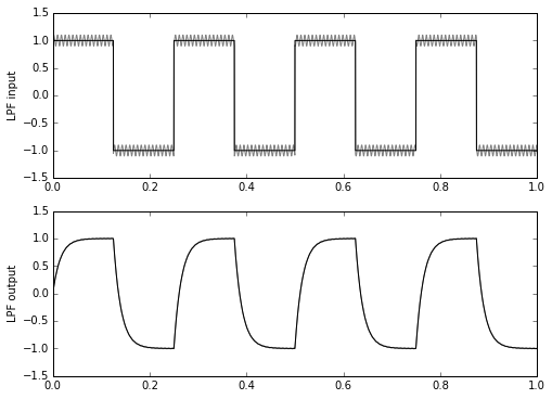
Now we’ll do a low-pass filter in fixed-point. We’ll plot the filter output (scaled back from integer counts to a floating-point equivalent), along with the error between the fixed-point and floating-point implementations.
# fixed-point low-pass filter

def lpf_fixp(x, alpha, Q, N, x0 = None):
    y = np.zeros_like(x, dtype=int)
    yk = x[0] if x0 is None else x0
    y_state = yk << Q
    alpha_scaled = np.round(alpha*(1 << Q)).astype(int)
    for k in xrange(len(y)):
        y_state += (alpha_scaled * (x[k]-yk)) >> (Q-N)
        yk = y_state >> N
        y[k] = yk
    return y

from matplotlib import gridspec

Q=12
x1q = np.round(x1*(1 << Q)).astype(int)
x2q = np.round(x2*(1 << Q)).astype(int)
Nlist = [6,4,2,0]
n_axes = len(Nlist)
for k,N in enumerate(Nlist):
    fig = plt.figure(figsize=(8,6))
    gs = gridspec.GridSpec(7, 1)
    ax = fig.add_subplot(gs[:6,0])
    y1q = lpf_fixp(x1q, alpha, Q=Q, N=N, x0=0)
    y2q = lpf_fixp(x2q, alpha, Q=Q, N=N, x0=0)
    y1qf = y1q*1.0/(1 << Q)     # convert back to floating point
    y2qf = y2q*1.0/(1 << Q)     # convert back to floating point
    ax.plot(t,x2,'#f0f0f0')   # show square wave for reference
    ax.plot(t,y1qf,'red',t,y2qf)
    ax.set_ylim([-1.1,1.1])
    ax.set_xticklabels([])
    ax.legend(('sq wave input','y1 output','y2 output'),loc='best')
    ax2 = fig.add_subplot(gs[6,0])
    ax2.plot(t,y1qf-y1,'red',t,y2qf-y2)
    ax2.set_ylabel('error')
    fig.suptitle('fixed-point lpf, alpha=%.6f, Q=%d, N=%d' % (alpha,Q,N))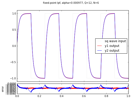
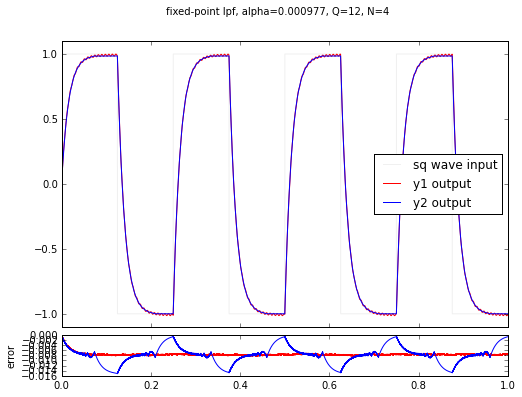
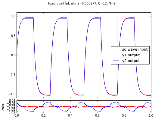
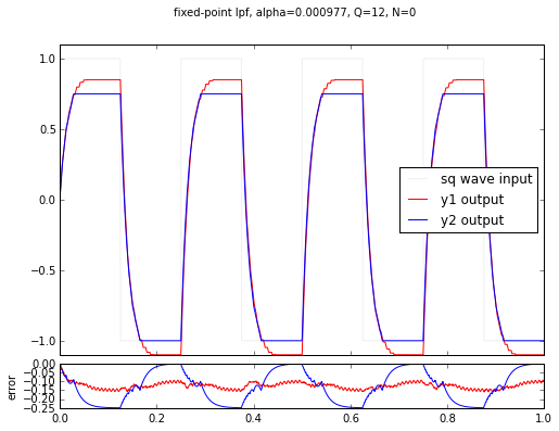
The proper number of extra state bits is \( N = -\log_2 \frac{1}{1024} = 10 \), but we used 6, 4, 2, and 0 in these examples. You’ll notice a couple of things:
- the lower N is, the worse the error gets
- for N = 6 the error is small but still present
- for N = 4, 2 and 0 the error is visually noticeable
- there is a DC bias: the output is always lower than the input. (This is true because a shift right represents a rounding down in the integer math.)
- the error for the y2 signal is always much higher; this is the output for the plain square wave with no harmonic content.
This last point is kind of interesting. The error caused by not having enough state bits is quantization error, and when high-frequency signals are present, it helps alleviate quantization error, in part because these signals are helping the filter state “bounce” around. This effect is called dithering, and it’s a trick that can be used to reduce the number of state bits somewhat. But to use it, you really need to know what you’re doing, and it also takes extra work (both up-front design time, and also CPU time) on an embedded system to generate the right dithering signal.
Aside from the dithering trick, you’re either stuck with using more bits in your low-pass filters, or you can use a larger timestep \( \Delta t \) so the filter constant \( \alpha \) doesn’t get so small.
Wrapup
Well, aside from the fixed-point quirks, the basic one-pole low-pass filter algorithm is pretty simple.
If you need more filtering than a one-pole low-pass filter can provide, for example you have lots of 1kHz noise on a 3Hz signal, another thing you can do is to cascade two of these one-pole low-pass filters (in other words, filter twice). It’s not as good as an optimally-designed two-pole low-pass filter, but it’s stable and easy to implement.
That’s it for today – happy filtering!
© 2015 Jason M. Sachs, all rights reserved.
- Comments
- Write a Comment Select to add a comment
A very nice write-up on single-pole IIR filter.
I guess many people will continue to read this post, so I would like to point out one thing-the cutoff frequency didn't get right. 1/tau is not the cutoff frequency in Hertz, but in rad/s, that is, omega=2*pi*f=1/tau, where omega is the frequency in rad/s. So when tau was selected to be 2msec, the cutoff frequency should be 80Hz instead of 500Hz. This would be clear if frequency responses of the low pass filters had been plotted. That is why I suggest, when designing filters, both of time-domain and frequency-domain responses should be simulated and analyzed.
Thanks for the nice post.

Alternatively, I could try to strip out text cells and publish the code as IPython notebooks; that's something that might be quicker.
It would be Mercurial, not Git -- while I use both (Mercurial for personal projects, Git for some things at work), and I definitely like Github best for code hosting, I just hate that Git occasionally shoves more complexity in your face when you try to do common tasks, and that the major Powers That Be (Github, and Atlassian via their Stash platform) don't support Mercurial as a simpler alternative that handles 99% of the cases you need in a DVCS. >:P >:P >:P

I like your peanut butter analogy.
Jason, I'm unable to read (understand) the code you posted here. But I'd still like to learn the material in your blog. Will you please translate the 'y += alpha * (x-y);' line of code into a standard difference equation using 'y(n)', 'y(n-1)', 'x(n)', etc. terms? I'd like to model that line of code using Matlab software. Thanks,
[-Rick-]
y[n] = alpha * x[n] + (1-alpha) * y[n-1]
Ah, Thanks. An "exponential averager." I should have figured that out on my own. Maybe your readers would be interested in the exponential averager material at:
http://www.dsprelated.com/showarticle/72.php
[-Rick-]
I thought that fft() converts from the time domain to the frequency domain, but that doesn't seem to be the case here.
I'm trying to understand the delta T term, in context of working with a sample buffer from the ADC, Is that the interval between samples. i.e., if I am sampling at 100Hz, delta T is simply x[n] - x[n-1] ?
Thanks!
Gary
Yes. If sampling at 100Hz, delta T would be 10ms.
If the incoming samples come in at different intervals, I guess it's enough to recalculate (or scale) alpha each time?
You can; there's a risk of the sampling jitter causing errors. (I don't have a source for understanding the math, unfortunately.)
Regularly-sampled systems are safer.
Yeah but also "regularly" sampled data might have (unknown) jitter. Or, I could switch to fixed rate sampling but, in practice, I'd get lower rates, especially if I need to control jitter; given this technique tends to perform better with oversampling, I'd be tempted to think "maximum rate" might still have advantages over "regular cadence rate". Of course I do not have any mathematical proof for this claim. Thank you for this article, it's so well written.
To post reply to a comment, click on the 'reply' button attached to each comment. To post a new comment (not a reply to a comment) check out the 'Write a Comment' tab at the top of the comments.
Please login (on the right) if you already have an account on this platform.
Otherwise, please use this form to register (free) an join one of the largest online community for Electrical/Embedded/DSP/FPGA/ML engineers:


