I have a continuous function that defines a 1D frequency domain signal.  Plot A in the attached image shows the real and imaginary portions of the sampled signal as a function of frequency inputs to the continuous function (64 data points in this case ranging from -5 to 5). This continuous frequency domain function is derived using the Fourier transform pair shown between plots A and B.  Using this pair I can get the spatial domain signal in Plot B which is correct.  However, I would like to be able to apply a discrete inverse FFT to arrive at the spatial signal.  Separately, using a FFT/IFFT algorithm adapted for the specific FT pair, I can go from the spatial signal with normal array indexing to the frequency domain signal shown in Plot C and back.  Clearly the frequency domain signals in Plots A and C look nothing like each other. How do I condition the sampled continuous function so that I can apply the inverse DFT to arrive at the desired spatial result?  Thanks for your time.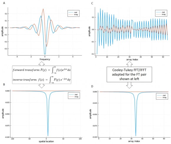

OK, so you started with curves A and by algebra and calculus you computed curves B which are the time response (you call it a spatial response, makes no difference here). Then it looks like the next step was to create figure D by sampling figure B. But you numbered the samples in D from 0 to 63. You assigned a sample number just a little more than 32 to the sample which has the greatest amplitude. That means it is essentially a pulse at around t=32. When you computed a DFT of that pulse you were selecting one complex exponential component in the frequency domain. That's what your curves C show.

Change the array index so that what you now have as 32 becomes 0, 33 becomes 1, ..., 63 becomes 31, and continuing modulo 64 you would have 64=0 becomes 32, 1 becomes 33, etc.

Now when you do the FFT (or IFFT) of the rotated curve C you will get something close to what you expected.

Comments:

OK, so you started with curves A and by algebra and calculus you computed curves B which are the time response (you call it a spatial response, makes no difference here). [Correct-JLeman] Then it looks like the next step was to create figure D by sampling figure B. [Correct-JLeman] But you numbered the samples in D from 0 to 63. You assigned a sample number just a little more than 32 to the sample which has the greatest amplitude. That means it is essentially a pulse at around t=32. When you computed a DFT of that pulse you were selecting one complex exponential component in the frequency domain. That's what your curves C show.

Change the array index so that what you now have as 32 becomes 0, 33 becomes 1, ..., 63 becomes 31, and continuing modulo 64 you would have 64=0 becomes 32, 1 becomes 33, etc. [I am not following, but will read up on modulo 64.  I have seen algorithms that shift frequency domain data, but have not seen that with spatial/time domain data.  As a side note, this is for electric field modeling so it is a spatial problem, but I agree that spatial/time makes no difference to the approach]

Now when you do the FFT (or IFFT) of the rotated curve C you will get something close to what you expected.

It should be a matter of a few seconds to do. Take the data in D, and create a new file which puts the last half at the front and the first half at the back, a 32 point circular shift. Then compute and plot the inverse FFT of the resulting file.

I agree with CharlieRader.  It is the assignment of the index number.

I find it vague to agree on index issues.

given any frequency domain vector if you do proper ifft then fft you get back to what you started with, without index changing.

I think your figure B is just wrong then you do fft of what is wrong.

kaz, this may help.  The only difference between the DSP of a real sequence and the inverse DFT of the same real sequence is a scale factor and the sign of the imaginary part of the answer.

So think about the DSP of a sequence which is approximately a pulse at approximately the halfway point of the sequence length. That DFT would be approximately (-1)^n. That's what the plot in C looks like. But if you look at A, you see a sine wave at a much lower frequency, whose DFT would be a pulse at a low frequency. Since the pulse in curve B (and D) is broadened out a bit, the sine waves in  A and C are "windowed".

I think the answer will be very simple if the OP sends those 64 data over as table or file here to the forum.

Post above in a reply to Platybek...signals.xlsx

Post deleted by author

The problem is related to electric field analysis. I have confirmed through independent means that figure B is correct from a spatial point of view. The calculus (continuous) forms of the FFT/IFT which convert between plots A and B are consistent.

Post deleted by author

When you go from the frequency domain (A) to the space domain (B) do you examine the imaginary part in the space domain?  The imaginary part should be zero in the space domain.  If there is a imaginary part in the space domain, it implies that the real part and the imaginary part are not symmetric/ anti-symmetric in the f domain.

I think if you consider the spatial domain as complex, you should get exact agreement.

cheers

Thank you for the reply.  The code is written in Julia and all numbers are complex, though as you say, the imaginary part in the spatial domain is zero (or very-very close to zero).

When you state 'FFT/IFFT algorithm adapted for the specific pair', what did you actually do?  I am unfamiliar with Julia, but probably can make some sense of the function calls.  Please show the lines for FFT and the IFFT calls.

Also, there is something fishy about C.  If the input in the spatial domain is all real, then the real part in the frequency domain will be symmetric, and the imaginary part would be anti-symmetric.  This clearly not the case in C.  This makes me suspect that there may be one or two terms that are not zero for the imaginary part in B. These aberrant terms would not be visible on a plot.  Please examine the actual numerical values around the symmetry points -- at the edges and around mid-point of the output data in B.

The attached pdf has supplementary info.  I try a different way of asking the question and I include some code snippets with examples of their function calls.  Fairly simple, but I need fast and lean. Thanks for taking a look - DSP is not my thing, but I've found it very interesting.

FFT_Question_Supplement.pdf

Since your data is only 64 samples please send the data for A B C and D.  I will take a look with Matlab.

cheers

This is the data for all four plots.  Plots without data for the horizontal axes are just indexed based on array position.  Thanks for the help.

signals.xlsx

if I do fft shift on your plot A vector then do ifft/fft and finally fftshift I get back your original input.

I don't see any issue but your plot B is wrong.

This is result of ifft of shifted Plot A , different from yours on plot B

I can get this as well, but this is the result obtained using the typical transform pair involving exp(i*2*pi*gamma*t).  Also, the imaginary component of the spatial (or time) domain result should be effectively zero.

Since  you obtained B by Fourier Transform of A (since you have computed with sampled data, there is really no difference between 'continuous' FT and FFT),you should be able to FFT the output (which is different from B) to reproduce A.  Do you?

Most likely you resampled (IFFT of A) to give the data you plot in B. There is a flaw in your resampling.  Let's consider a real data  series x with total number of points N.  When N is even (say 8), the symmetry points are 0 and 5.

the first point x(1) is not repeated in x(8).  The symmetry point is x(5), with 3 points on either side, excluding x(1). (I do not what Julia convention is, Matlab does not allow an index to be 0, Matlab arrays start at 1, causing perpetual confusion). For even value of N, the symmetry point is a sample, in this example for N=8, it is x(5). In the data you have given for both A & B, the symmetry point is between 32 & 33 row.

Regardless of B to C operations, you should be able to get A from B by FFT.  You do not have to reindex or resample. Just pass the output of IFFT(A) as the input of FFT, you shhoulod get exact A.

I obtained B by inverse Fourier transform of A.  My code implements what I'm calling the continuous form because it integrates the original continuous frequency function (a type of Bessel function) over +/- infinity to get each data point in the spatial domain. I simply do that calculation 64 times to get the data in plot B. Plot A is showing 64 samples of the original continuous frequency domain Bessel function. So I can get B from A using the continuous inverse transform and A from B with the forward continuous transform.

However, when I take the sampled array corresponding to B and apply the discrete FFT, I get plot C

Adding to this - the integration method is quite slow which is why I'm trying to do this by discrete methods.  When it is all said an done I would like to understand how to recondition the indexing of A to be able to get C with an inverse DFT.  I'm confident that plots for A and B/C are correct.

You have said several times that you are sure that the computation from A to B is correct. We are not sure, however, that we understand the sense in which you mean correct. A describes a continuous function of frequency. What you show in B seems to be a continuous function of frequency but you have only computed it at 64 points, not infinitely many points. That may be OK, but when you take the inverse FFT of a sequence of 64 points, you are computing the Fourier transform of a different function. It is different in two ways. First, it is sampled. Second, and often more important, it is a periodic repetition of the original(A) function. You won't see the repetition because only the first period is shown. 

Thanks.  I think I see what you are getting at. A lot of good responses on this forum. I need to let all this information simmer and sink in.

"I have a continuous function that defines a 1D frequency domain signal."

Let's stop right there.  In the frequency domain you have a spectrum.  Numerically the same as a signal, but conceptually, that is a non-sense statement.

The others are correct as well.  My advice is use an odd number of points, then you can map the [0,N-1] spectrum to [-(N-1)/2,(N-1)/2] with DC at the center and no worries about splitting the Nyquist bin.

My answer here at another forum may also help clarify a few things conceptually:

Amplitude after Fourier transform

Fair enough.  Poorly worded on my part.  Plot A is spectrum plot.  Thanks for the link.  I will review.  It looks helpul at first glance.

You're welcome.  It's so easy to be misled when the proper terms aren't used.  Having said that, the forward and reverse FTs are only distinguished by a negative sign in the right spot (and normalization factor, depending on how you define it).  Behaviorally the are the same, so what applies one way, applies the other in terms of properties.

You may find the question and my answer here How to get Fourier coefficients to draw any shape using DFT? somewhat pertinent, and even interesting.

I reviewed your answers in the other forums and I think they do relate to the specific concepts I am confused about.  

Taking a step back, attached is a better description of the continuous problem I am looking at. 

Explanation of Analytical Equations.pdf

Disregard the items I previously posted in the thread. In code I can implement numerical integration over +/- infinity (effectively) and thus can go back and forth between the spatial and frequency domains.  I do this via a numerical approximation of the continuous Fourier transform equations, not with a true discrete Fourier transform or inverse discrete Fourier transform. The method I am using is slow and fine accuracy is not necessary. I expect a true DFT/IDFT method would be much faster.

In the end, the continuous analytical expression for the spectrum is a given.  I am trying to figure out how to sample this function and arrange indexing so that I can apply an inverse DFT to get an approximation of the spatial domain result.  Note that since this is one point charge in space, the problem is aperiodic. I see the correlation between the continuous and discrete in your other responses, but am struggling to get this to work. If you have any suggestions given this specific case I'd appreciate it.     

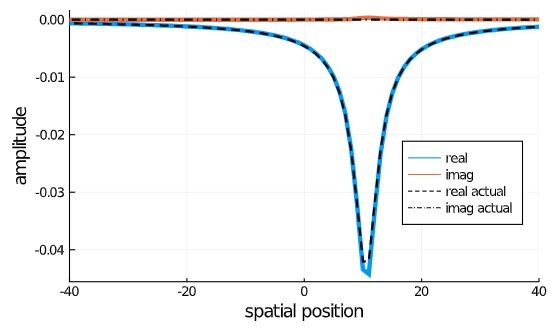
It looks like from your "spatial location" chart that you are looking for a real valued solution.  A property of the DFT is that the bin values for real valued solutions come in conjugate pairs.  That is

X[N-k] = X^*[k]

You will notice that in your chart as well.  The blue line is an even function and the orange line is odd.  You should be able to map the DFT bins 0 to N/2 on your domain of 0 to 3, then N/2 to 0 on your domain of -3 to 0.  I'm just emphasizing you need to place the DC bin in the center.

In case you might be off center my a smidge and are getting some imaginary results, you could conjugately average your supposed to be conjugate pairs to make true conjugate pairs.

This should give you a good approximation making sure you have an N large enough to handle the curves.

Do you mean:  ...You should be able to map the DFT bins 0 to N/2 on your domain of 0 to 3, then N/2 to N on your domain of -3 to 0...?

Yeah, sorry, rush job.  N isn't in the DFT, so up to N-1 if you will.  But N would align on 0.

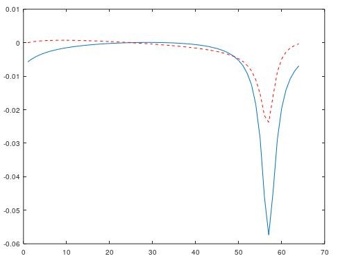
Ok. That makes sense and I was able to get things to work.  I had to experiment a bit and I'm not sure I quite matched your description above, but the attached diagram below (see link: FinalResult.jpg) shows the approach I used.  Maybe this is what you meant. I had to reverse the order of the reassembled spectrum array to get the spatial offset to be on the correct side. This is the part that didn't seem to match your description.  

FinalResult.jpg

zoomed-in version of the last plot:

Three questions if anyone has time to consider an answer:

First Question

Usually when performing the inverse FFT it is my understanding that the final result of the inverse must be divided by N.  I did not have to do that in this case.  Any idea why?  Perhaps that is only necessary when doing both the forward FFT and reverse FFT together? 

Second Question

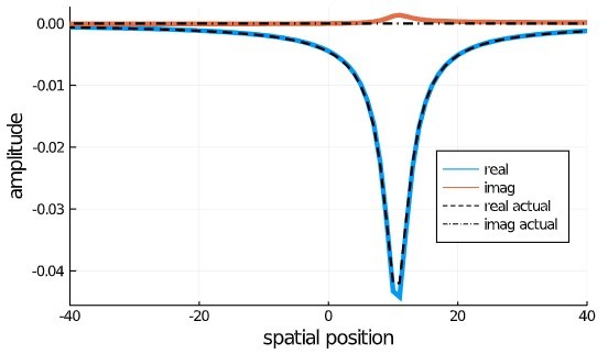
I'm struggling a bit with how to increase spatial resolution. The final results above are achieved with 1024 samples in the frequency domain.  The image below is with 4096 samples. The error in the imaginary component is lower, but I don't have finer resolution in the spatial domain - it just gives me more distant extents (not shown since the plot is zoomed).  Is there anything I can do on the frequency domain side so that I have better resolution in the spatial domain?

Last Question

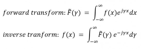
In the end I used the IFFT function of the FFTW code (fftw.org) which is based on the following FFT/IFFT pair:

forward: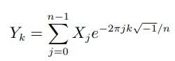

revers: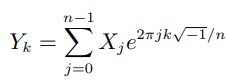

The original continuous frequency domain equation was derived using a forward Fourier transform from this pair:

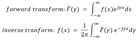
Note that the arguments of the exponential terms between the two pairs are of opposite sign and differ by the 2*pi multiplier. I expected I would have to adapt the discrete case by changing the exponent sign and removing 2pi to make it consistent with the corresponding forward transform used to derive the original equation. I think this was part of my problem all along as I was using an adapted equation. However, I reverted to the original FFTW version for some experimentation and found it worked.  

Any idea why the consistency between transform pairs was not necessary?

You've done well.  There are three common conventions for normalizing the DFT.

1) 1 forward 1/N backward

2) 1/sqrt(N) forward, 1/sqrt(N) backward

3) 1/N forward, 1 backward

#1 is the most common, and I think wrong.  #2 is the mathy one as it makes the DFT a "unitarian transform"  #3 is the right one in my book (oops don't have a book, so if you prefer the first link I gave you or read my articles here Cedron Dawg's DSP Blog)

Libraries, like FFTW, will not normalize at all and leave the decision up to you.  The also save a multiplication that way.

The "how to draw DFT" link answers your resolution question.  You can interpolate by zero padding the source.  Now that you have figured out where N is on your scale (lookup fftshift if using MATLAB, I'm a nonuser)  Double, or more or less, your N and fill your values [0 to limit 0000000000(Nyquist=0)0000000000 -limit to N-1], then take the inverse.

Your alternative to doing zero padding in the frequency domain is to recognize that the bin values in a 1/N normalized DFT are the coefficients of the Fourier series to reconstruct your spatial signal.  This is also known as the "trigonometric interpolation polynomial".  (Which people extrapolate and then claim "The DFT assumes the signal repeats itself outside the frame.)   If you say "acts as if" then you are okay.

With these coefficients you literally have the definition of the continuous function that passes through all the points and can zoom down to an level of detail you want.

See:  
Using fourier coefficients to reconstruct data in matlab As you can see, I'm not shy about expressing my opinion on this normalization thing.  (Warning, in this answer one full frame is \(2\pi\).)

That first link I gave is one of the best answers I have ever done, I think everybody should go read it (and you reread it now that you're better oriented).

The DFT is defined on the interval 0 to 1 in the continuous domain in my mapping there.  You can't just shift it to the left by 1/2, instead you need to slice it at 1/2 then shift that piece one entire interval to the other side of zero.  Now you are zero centered.  The DFT definition and implementations go 0 to N-1, honestly the formula doesn't care what order you do the calculations in.

Aliasing it technically what allows you to shift a piece of the DFT any number of whole frame widths.

  X[-1] = X[N-1] = X[2N-1]

If anybody wants to argue that 1/N is not the most sensible normalization, bring it on.....

Excellent!  Thanks for the help.  I'm in power systems and never expected to delve into the DSP realm. However, it has been very interesting.  

It seems the result I am getting supports your statement regarding the third convention for normalizing since the forward portion of the FT was done using the continuous form and no 1/N was necessary for the inverse.

I was able to get the zero-padding option to work.

Good.  These are extremely powerful tools in the right situations.  I think upon review, the original answers are going to look excessively clear.

Power systems? as in Hydraulics?

Oh, boy.  I'm just going to shout "DFT used in control theory" and run.

Have fun.

Negative - power systems.. as in high voltage transmission line electromagnetics.  I don't work in controls, but am aware that much DSP is involved in that area of the industry. 

Hello jleman: looks like you have had most of your questions answered.  Since you are in DSP learning mode, perhaps it is useful to restate some basics:

1. A sampled dataseries, whether in time (space) or frequency domain is always periodic, i.e. equivalent to Fourier Series.  What you see in the time is one period. If start out with N data points in time domain, you get N coefficients in the freqwuency domain. Regardless of the name Fast Fourier Transform always uses Fourier Series.

2. The FFT is just a fast algorithm to compute Fourier Series, if N is a product of small prime numbers.  It is most efficient when N is a power of 2, it is also quite fast when N can be factorised into small prime numbers.  FFT is snails pace when N itself is prime.

3. When the input is an all real data series, the output of FFT, as a result of the algorithm, comes out in a specific order of the frequency coefficients.  For lack of a better name, we call it FFT symmetry.  Consider a all real time series x(k), k=1 to 8, and the FFT output X(n), n=1 to 8.  X(1) is the DC term. (Since you are in the Power industry, you will appreciate that DC stands for Direct Current.)  The DC term, just the mean, is all real (no imaginary).  The next N/2 = 4 terms represent the +ve frequency coefficients.  The last term X(5) is at the Nyquist frequency and is all real. X(6), X(7), X(8) are the conjugates of X(4), X(3), X(2) respectively.  You notice that  the DC term X(1) and the Nyquist term X(5) do not have conjugates.  Also the first point is not repeated at the last point, both in time and frequency domains.

4. In your data for A, in the frequency domain, you did not have FFT symmetry.  You also did not have a DC term, which should have been between your frequencies  -0.079365 and 0.079365. Since in the real part of your data, this is an extremum value, it may be significant, and you should recompute the frequency domain data.  The imaginary part here will be 0.

5. Unless your dataset is quite large, it is not necessary to strive for a N that is a power of 2.  As long as N is small, FFT will deliver,  the fastest possible. For a prime N, FFT will compute at snail's pace. 

6. You probably have the answer to your original question: You computed (you thought) B after Fourier Transform of A.  But when you FFTed B, you got C instead.  I think if you go through all the steps, you will get a transform of A that is similar to your current B, but significantly different.  But you will see that A and B are a FT pair.

Good luck

Thank you.  That is very helpful.  I will review this information in more detail next week, but two questions come to mind:  1) speed is important in my code so I would prefer to use an array that is some power of 2 (I've noticed a factor of 10 improvement in speed when I do) However, if I include the DC term at freq = 0, doesn't that make the array an odd size (some 2^n + 1).  Or do you still keep the array size at 2^n and not worry about having the same range of points above and below freq = 0?   

The second question has to do with the 2*pi.  The original continuous spectrum equation was derived using a Fourier transform pair that did not include the 2*pi in the exponential term.  I would have expected then, that the corresponding inverse DFT would be based on a form that likewise did not include the 2×pi. However this was not the case.  The FFTW code that worked used the standard inverse form with the 2*pi.  Any ideas why that would be the case?

I didn't notice Platybel's observation that you were missing the DC component in your data.  You've tried zero padding, maybe you should try zero insertion.

Another parlor trick if you will.  Here is an article that explains the principle in the reverse direction.
Why Time-Domain Zero Stuffing Produces Multiple Frequency-Domain Spectral Images

The missing DC value shouldn't be that big of a deal as it will be "interpolated" inherently with this operation.  Take your balanced values and stick them in Bins 1 and -1, and work your way outward, filling only the odd bins.  Bin -1 is bin N-1 as you have now figured out.  Assuming of course your values are balanced that way.

You may want to go back to source and make sure your sampling scale includes 0 (DC) and is balanced around that.  After the inverse DFT, your resultant imaginary values should be zero (within numerical precision).

The problem with the zero insertion is it makes the DFT bigger/slower.

If you know that your negative frequency integral calculations are supposed to give you the complex conjugate value of the postive one, there is no point in calculating it.  Start with DC in bin 0, your first freuquency step in bin 1, and put its complex conjugate in bin N-1, up to your limit.  Leave some zeros in the center to suit your taste and you should have the fastest way to do it.

The normalization factor issue is similar to the forward case.  Note $$ \gamma = 2 \pi t $$

Hello jleman: I posted a reply about 6:30am today (about 9 hours ago), but it seems to have vanished.  So I am retyping it in shorter form.  

If dropping a point or adding a point does not detract too much from the information content, and makes the fft speedier it is OK to do so.  Remember that whenever you are dealing with a sampled data set, it is periodic, both in t and f domains. x(t) and X(f) are just one period. For your data in A, dropping one end point where both real and imaginary parts are tending to zero, will not make a significant difference.

You have raised the question of 2*pi.  There is a lot of confusion.  Perhaps an example with a synthetic data series x(t) will help. The goal of X(f)=fft(x(t)), is to give you the Fourier coefficients,  Similarly the operation ifft(X(f)) should give you back x(t) exactly. So

Let x(t)=3+1*sin(pin*t)+2*cos(2*cos(2*pin*t)+3*sin(3*pin*t)+4*cos((N/2)*pin*t), where pin=2*pi/N, and we consider N=8. We have

the known coefficients = 3,1,2,3,4 (I am considering the amplitudes of cos and sin terms together)

x(t)=9,1.83,3,1.83,9,-3.83,7,-3.83

fft(x)=X(f)=24,-4i,8,-12i,32,12i,8,4i

|(X(f))|=24,4,8,12,32,12,8,4  These clearly are not the input coefficients.  If we divide |X(0)| and |X(N/2)| by N, and the other terms by (N/2), we get the right values. 

So if you have determined X(f)fft(x(t)), in order to determine the Fourier coefficients,  you have to have one further step to obtain the Fourier coefficients.  The forward fft and the inverse ifft do not include the division by N or N/2.  Note in the finite Fourier transform N=2*pi.

In your case, for A, you have computed the complex Fourier coefficients, and have included the division by N or N/2 in your computation.  In order for you to use the ifft on dataset A, you have to bring it to X(f) format with multiply by N or N/2 the appropriate terms before applying ifft. 

Just to clarify: To obtain Fourier coefficients from X(f), you have to divide by N or N/2.  If you have the Fourier coefficients, you have to reverse this step by multiplying by N or N/2.  The only terms to be operated on by N are the X(0) and X(N/2) terms, if N is even. If N is odd then N operates on only X(0).  All other terms, for both N odd and N even, are operated on by N/2. 

So you have to execute following steps: (1) compute value for 0 spatial distance. This will alter the intersample distance between 0 and the two neighbouring samples; (2) recompute other spatial values, or try to obtain fft interpolated values; (3) rearrange your data fit fft symmetry; X(0) first, then X(1) to X(32) (the positive frequencies), then the -ve frequencies to make N=64 terms; (4) Multiply X(0) and X(32) by N, the remaining terms by N/2; (5) Now apply ifft.

If N is odd,  say 9, you operate on just X(0) with N, and all other terms with N/2.  This will apply if you use N=65.  I siggest you try this out, just to convince yourself.

I trust all your questioned have been finally answered.

Good Luck.

Thanks for taking the time to type this up, twice apparently.  Much appreciated.  The examples help a lot.  I'll be working through this today.  

And thanks to other folks who posted - those conversations helped get me oriented.