


Understanding the Comb Filter Frequency Response
I have some troubles understanding the comb filter. Hope someone can help.
I am going to use the following figure to illustrate my questions:
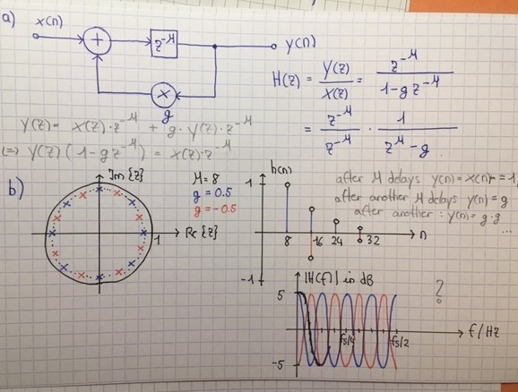
You can see the block diagram of an M-fold comb filter with feedback loop. Let's have a look at the pole-zero plot: Poles should be wherever the denominator of the transfer function becomes zero. That is whenever z^M = g. For the given example this happens at z = g^(1/M) = 0.5^(1/8) = 0.917. Of course we will have M poles and therefore can just equally space these on a circle with radius 0.917.
Now, how do we plot the impulse response? We simply have a look at the block diagram and send in a dirac, or better say a unit pulse. The 1 occurs at the output after M=8 delays. Since we do not insert another input, the output will be fed back after 8 delay steps, but it is multiplied by g. So at n=16 the output equals 0.5 ...
But how can we derive the frequency plot from all of this? Why does the frequency plot look the way it does? How do I know the magnitude equals 5 dB and how do I know I will have a sine-wave shape that has 4 periods until fs/2 ?
Can somebody explain this to me, please?

You may want to start with this here on the site:
https://www.dsprelated.com/freebooks/filters/Analy...

I am a bit confused. Is this comb or Integrator. How come you add such long delay to feedback and why. also you rightly say about impulse input but then move to describe sine waves.
You need to explain your questions better so you get answers

It looks like you have already computed the transfer function H(z) in z-domain. To compute the frequency response, you can simply set z = e^{jw) and compute H(e^jw). This will be a complex function of w, from which you can compute the magnitude and phase response. Also, w = 2 pi f, so you can interpret the frequency response defined over 0 <= w <= pi, or equivalently 0 <= f < = 1. Keep in mind that this is the normalized frequency, i.e. the actual frequency range [0, fs/2] has been mapped to the normalized frequency range [0, 1].
In your case, H(z) = 1/(z^M-g). If you set z = e^jw and compute the magnitude response, you get:
|H(e^jw)|^2 = 1 / (1 + g^2 - 2gcos(Mw))
You can plug in g and M and plot it vs. w for 0 <= w <= pi to see what you get. It looks like you should get 6 dB at w=0 and not 5 dB...

Hi Luk_11. For u = 8 & g = 0.5, your network's frequency magnitude response (on a linear vertical axis and a freq axis that goes from minus half the sample rate -to- plus half the sample rate in Hz) should look like the following:
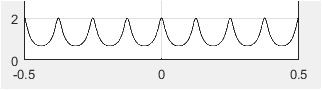
The network's gain at zero Hz (DC) is 2. The bottom of the valleys in the freq magnitude response are 0.666, which is roughly -9.5 dB below the peaks.
thx a lot, Rick!
There is a figure on wikipedia: Comb Filter Frequency Response
And it says: The peak value (on a linear vertical axis) equals 1/(1-g), so for the given example of g = 0.5, it is 2. It also says: The peaks repeat at integer multiples of 1/M, where M is the delay. So in my case, M=8, I would expect repetitions at 1/8 pi, and so on, for a horizontal axis that gives Omega. But I think that's wrong, as in the given figure M=2 and repetitions do not occur at 1/2 Omega, 1 Omega, 3/2 Omega. I don't see what I missunderstood, though.
Also, I would rather have this in dB on the vertical axis and f in Hz on the horizontal axis
Hi Luk_11. Your confusion is NOT your fault.
The freq axis in the wikipedia spectral plot is incorrect. (Although I avoid such vulgarity, today's young people would say, "WTF!")
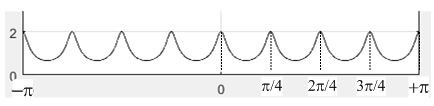
For the wiki spectral plot to be correct we have to divide its freq axis values by K = 2. Doing that we see that when K = 2 there are spectral peaks at multiples of 2*pi/K = 2*pi/2 = pi rad/sec. The wiki variable K is your variable mu. So, after changing the freq axis labeling in the spectral plot I posted above, when your mu = 8 the spectral peaks occur at multiples of 2*pi/mu = 2*pi/8 = pi/4 radians as shown below:
allright, thank you so much, Rick!
Hi,
I can propose another way to understand how to build the spectrum of a comb filter, either recursive or not, and also its impulse response.
1. Study of unit delay cases
First of all, you need to study the spectrum of cases with a unit delay and determine the nature of the related filter.
For the recursive filter, we can just study the filter :
y[n] = x[n] - a.y[n-1],
where a is a real within ]-1, 1[ to consider only the stable cases.
With the z-transform we have :
Y[z].(1 - a.z^{-1}) = X[z]
so the transfer function is
H[z] = Y[z] / X[z] = 1 / (1 - a.z^{-1}),
which can also be rewritten:
H[z] = (z - 0) / (z - a).
Considering the restriction to the Fourier digital domain, that is to say the unit circle defined by z-> e^(2 pi j nu) with nu the reduced frequency given by nu = f / Fs, we have the following expression for the gain:
|H[nu]| = | e^(2 pi j nu) - 0 | / | e^(2 pi j nu) - a|.
Introducing the relation between complex numbers and mathematical affixes, we can consider the origin point of the z-plane O(0), the pole point P(a) and a moving point over the unit circle M(e^(2 pi j nu)).
So, we can interpret |H[nu]| as the ratio of distances OM and PM.
As OM is always equal to 1, |H[nu]| = 1 / PM.
11) 0<a<1
If 0<a<1, the point P is on the real axis within the ]0, 1[ interval.
PM passes from 1-a to 1+a when nu goes from 0 to 0.5 (Nyquist frequency), so the gain decreases when nu increases. And, as the modification of PM is tiny when nu is in the vicinity of 0 and also in the vicinity of 0.5, we have horizontal tangents when nu equals 0 or 0.5.
So, the filter is then a low-pass one for 0<a<1 when nu is within [0, .5].
As the Discrete Time Fourier Transform (DTFT) satisfies the hermitian symmetry, |H[nu]| is an odd function.
As the DTFT is periodic with a unit period in nu, |H[nu]| completed by parity within the [-.5, .5] interval is periodic over R.
12) -1<a<0
Now, the P point is still on the real axis but within the ]-1, 0[ interval.
PM passes from 1+|a| to 1-|a| when nu goes from 0 to 0.5, so the gain increases which nu. And we still have the horizontal tangents for nu equals 0 and 0.5.
So the filter is a high-pass one for -1<a<0 when nu is within [0, .5].
We still have 1-periodicity and the gain parity (due to hermitian symmetry) so |H[nu]| completed by parity within the [-.5, .5] interval is again periodic over R.
13) non recursive unit-delay comb filter
One may follow the same process but with a new difference equation:
y[n] = x[n] + b.x[n-1].
It is also necessary to distinguish the positive and negative cases for b and using the link between complex numbers and z-plane points makes the study rather easy.
2) from the unit delay to the D_0 delay
21) the principle
I will only describe the case of the recursive comb filter for 0<a<1 but the principle is the same in all cases.
When we change the value of the delay from 1 to D_0 (with D_0 an integer greater than 1), each "echo" generated by the retroaction (multiplied by a) is delayed.
For the unit delay, the echo of unit impulse applied at the input of the filter gives (after its apparition at the output for sample 0), an echo with a value for sample 1, an echo with a^2 value for sample 2, an echo with a^3 value for sample 3 and so on.
For the D_0 delay, each echo is delayed: first echo appears at sample D_0 with a value, second echo appears at sample 2D_0 with a^2 value, third echo at sample 3D_0 with a^3 value and so on.
So when considering the transition from the unit delay impulse response to the D_0 delay impulse response we constate that we have a time dilatation of factor D_0.
But, if we have a time-domain dilatation of factor D_0, we also have a time-frequency compression of factor D_0! And this is the conclusion which mut be used to build the filters spectra.
22) building of the spectra according the D_0 value (0<a<1)
For D_0=1, we have a low-pass spectrum when nu is in [0, 0.5], and, parity and 1-periodicity in nu.
For D_0=2, we compress the spectrum with a factor 2, so we find again the low-pass behavior for nu in [0, .25] but we also have for nu in [0.25, 0.5] the unit-delay filter spectrum part formerly associated with nu in [0.5, 1]: the symmetrical of the [0,0.5] part of the spectrum with a symmetry according nu=0.5.
In fact, when performing the frequency compression of factor 2, we take into account the next semi-period of unit-delay spectrum.
For D_0=3, we apply a frequency compression of factor 3. We then find again, for nu in [0,0.5] for the 3-delay comb filter, the part of the 1-delay comb filter spectrum within [0, 1.5].
In fact, when performing the frequency compression of factor 3, we finally have 3 semi-period of the 1-delay spectrum within [0, 0.5].
In fact, each time we increase the D_0 delay with 1, we also increase the number of semi-periods of the 1-delay spectrum taken into account within [0, 0.5] to build the D_0-delay comb filter spectrum.
We are then able to access, for instance, to the spectrum give by Rick Lyons
It is the simplest method I have found to explain the comb filtering principle to my students.
I hope it may help.
Laurent Millot


