Hi.
Two weeks ago I posted a Forum message:

https://www.dsprelated.com/thread/8675/is-this-tim...

showing a video of oscillating pool ball pendulums. Because that Forum message generated a moderate amount of interest, and I wanted to study what I thought was peculiar behavior in the swinging pool balls, I wrote a MATLAB routine to duplicate the video as a MATLAB animation. (I had a colleague try to modify my code so it would run under OCTAVE software, but he wasn't able create a usable OCTAVE version of my code.) In case anyone's interested, here's my MATLAB code for the pool ball pendulums:

function [] = pendulums_of_pool_balls
% Richard (Rick) Lyons, June 10, 2019
clear; clc,

G = 9.81; % Gravity constant (here on Earth)
Num_Balls = 15 % Number of pool balls
T = 10; % Total "computer time" period of oscillating pool balls
Plot_Strings = 'Y'; % 'Y' to plot strings, 'N' for no strings

First_Ball_Freq = 50;  % Longest-string pendulem's Osc. freq
Last_Ball_Freq = 50 + Num_Balls-1;  % Osc. frequency delta = one
Freqs = Last_Ball_Freq:-1:First_Ball_Freq;
Freqs = Freqs/T; % Reduce frequencies by a common factor
String_Lengths = G./(4*pi^2.*Freqs.^2); % Lengths of pendulums' strings

K = sqrt(G./String_Lengths); % define pendulums' dynamic parameters
t = linspace(0, 10, 1200); % Time variable

    %%%%%%%%%%%%%%%%%%%%%%%%%%%%%%%%%%%%%%%%%%%%%%%
    % Plot a single snapshot at time 't' if you wish
    %%%%%%%%%%%%%%%%%%%%%%%%%%%%%%%%%%%%%%%%%%%%%%%%
    Q = 5; Delta = 0.0000; % Set Delta to zero or a small value
    %t = linspace(10/Q-Delta, 10/Q-Delta, 1); % A single instant in time

Half_Swing_Deg = 5; % Max half swing angle in degrees
Theta_Max = Half_Swing_Deg*pi/180; % Max half swing angle in radians

% Compute X/Y position of ball based on equation for a circle
Len_Squared = String_Lengths.^2;

for N = 1:Num_Balls % Outer loop, Number of balls
    
    for M = 1:length(t)
        Theta(M) = -pi/2 + Theta_Max*sin(K(N)*t(M));
        X(N, M) = String_Lengths(N)*cos(Theta(M));
        Y(N, M) = -sqrt(Len_Squared(N)-X(N, M).^2);
    end
end

% Define max & min X/Y axes for plotting
Max_Len = max(String_Lengths); Max_X_Axis_Swing = Max_Len*sin(Theta_Max);
X_Axis_Min = -1.1*Max_X_Axis_Swing; X_Axis_Max = 1.1*Max_X_Axis_Swing;
Y_Axis_Min = -1.0*Max_Len; Y_Axis_Max = -0.9*min(String_Lengths);

% Define ball color vector Numbers
Colors(1,:) = [0 0 0]; Colors(2,:) = [0 0 1]; Colors(3,:) = [0 1 0];
Colors(4,:) = [0 1 1]; Colors(5,:) = [1 0 0]; Colors(6,:) = [1 0 1];
Colors(7,:) = [1 1 0]; Colors(8,:) = [1 1 1];
for Loop = 1:Num_Balls;
    ColorNum(Loop) = mod(Loop, 8) + 1;
end

% Start the animation
Computer_Time = round(1000*t)/1000;
figure(1), clf
MarkSize = 10; % Size of plotted balls

for Loop = 1:length(t)
    plot(X(1, Loop), Y(1, Loop), 'o', 'MarkerFaceColor',...
                          Colors(2,:), 'Markersize', MarkSize)
    hold on
    for LoopLoop = 2:Num_Balls
        plot(X(LoopLoop, Loop), Y(LoopLoop, Loop), 'o', ...
            'MarkerFaceColor',Colors(ColorNum(LoopLoop),:), ...
                                          'Markersize', MarkSize)
        if Plot_Strings == 'Y'
            plot([0, X(LoopLoop, Loop)],[0, Y(LoopLoop, Loop)],...
                  ':k') % Plot pendulum lines
        else, end
    end
    hold off
    axis off
    axis([X_Axis_Min, X_Axis_Max, Y_Axis_Min, Y_Axis_Max])
    grid on, title(['Computer time: t = ',...
        num2str(Computer_Time(Loop))])
    pause(0.001); % A short pause is necessary
end

Rick-

With this are you able to answer the aliasing question ?  Also can Matlab create an animated gif that you can post somewhere and we can see ?

-Jeff

Hi jbrower. Watching the original pool ball pendulum video, it looked to me that the instantaneous East/West positions of the balls was VERY similar to the amplitudes of discrete samples of a continuous chirp signal being digitized by an A/D converter.

I haven't explored that notion because I've been distracted by trying to figure how many times, and when in time, do groups of the pool balls "line up" with each other. Stated in different words, I tried to figure how many times, and when in time, do groups of the pool ball strings all have the same Theta displacement angle relative to a vertical line. (You can see this in the video. At 26 seconds into the video there are four sets of balls lined up with each other. At 33 seconds into the video there are three sets of balls lined up with each other.) I've been studying that behavior but the results of my study are so weird, so unpredictable, that I'm afraid to tell anyone what I am learning! (Not that anyone cares.)

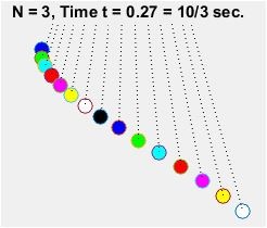
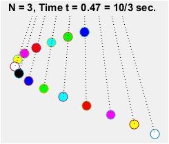
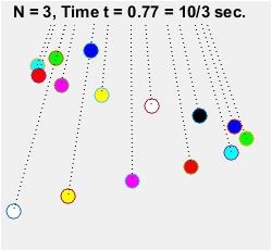
You asked about generating MATLAB animated gif files. Now that's a subject that I need to learn. (I found a tutorial web page on that topic but I haven't yet read that web page in detail. Later I'll let you know what I learned from that web page.) In any case jbrower, to give you a notion of what my MATLAB code does, the following are "snapshots in time" of the animation produced by my MATLAB code.

 

Rick-

First the snapshots look good.  Seems you indeed have the simulation working correctly.

To confirm your chirp theory, you can add spectrogram type output to your MATLAB simulation, taking the ball positions as discrete samples in time.  It would be very interesting to see a 2-D spectrograph with sliding FFTs and Hanning window, and see just what those positions look like over time.

If you did that, it would answer the "when do they line up" question, as you would see a null (dc) in the spectrograph.

-Jeff

Hi Jeff. I just saw your June 13th post five minutes ago.

Your idea of a spectrograph is a good one! Thanks. I will explore that idea.

Hi Rick,

Pendulums have periodic motions which approximate simple harmonic motion.  The difference is $\theta$ vs $\sin(\theta)$ in the guiding differential equation.  At small angles these are close approximations of each other.

The important point is that they are periodic and the period is dependent on the string length.  Thus you can define any period you want by picking the right length string.  Any old fashioned clockmakers here to back me up on this?

So, to build an assemblage of pendulums, you simply need to define the first one and how many periods you want it to swing.  That will define a time frame.  Suppose you decide on S swings in your time period.  For the next pendulum, shorten the string somewhat so it swings S+1 times in the same time frame.  These two will now line up only at repeat times of your time frame.

Next, add another pendulum with a slightly shorter string that swings S+2 times in the same time frame.

And so on, up to fifteen for the full billiard ball set.

As I said before, they are very much like the basis vectors in a DFT.

The same effect (with true harmonic motion) can be produced by having ants run in circles around a common center at the same speed with varying radiuses.  The outer ant does S rotations in some time frame.  The next inner ant does S+1, the next S+2, etc.  It is just a matter of calculating the correct radius, similar to the problem of finding the right string length.

Ced

Hi Cedron. I'm familiar with the ideas you presented. Your words correctly describe the purpose of the commands in my MATLAB code. To model the pendulums' motions, your have three choices:
[1] Increment the balls' periods by one,
[2] Increment the balls' string lengths by one, or
[3] Increment the balls' frequencies by one.

Only choice [3] is correct to simulate the original video I posted.

A BIT OF PENDULUM TRIVIA:
In the 'theta ≈ sin(theta)' approximation you mentioned, theta is the maximum angle a pendulum's string makes relative to a vertical line. In my MATLAB code I set that maximum theta (variable 'Half_Swing_Deg') to 5 degrees which is the typical maximum theta used manufacturers of grandfather clocks.

As far as when they line up -- if they're simple harmonic oscillators, then each will have a period p_n, and they'll line up when there's a set of integers N_n such that p_n * N_n equals some constant.

If they're typical pendulums that aren't quite linear harmonic oscillators, and if they don't interact, then it's way more complicated, and possibly not solvable symbolically.

If the bar they're suspended from isn't perfectly rigid, or if they "talk" to each other via the wind (which should be a thing given how close they are to each other) then the dynamics would get really complicated, and possibly even chaotic.

Very cool, Rick.

Below you will find Rick's original function with 5 commands added that generate an mp4 video of his animation.

I will try to attach the generated mp4 file, as well.

___________

I don't think that it worked.  11MB may be too much.

---

function [] = pendulums_of_pool_balls

% Richard (Rick) Lyons, June 10, 2019

clear; clc, 

G = 9.81; % Gravity constant (here on Earth) 

Num_Balls = 15 % Number of pool balls

T = 10; % Total "computer time" period of oscillating pool balls 

Plot_Strings = 'Y'; % 'Y' to plot strings, 'N' for no strings

First_Ball_Freq = 50;  % Longest-string pendulem's Osc. freq

Last_Ball_Freq = 50 + Num_Balls-1;  % Osc. frequency delta = one

Freqs = Last_Ball_Freq:-1:First_Ball_Freq;

Freqs = Freqs/T; % Reduce frequencies by a common factor

String_Lengths = G./(4*pi^2.*Freqs.^2); % Lengths of pendulums' strings

K = sqrt(G./String_Lengths); % define pendulums' dynamic parameters 

t = linspace(0, 10, 1200); % Time variable

    %%%%%%%%%%%%%%%%%%%%%%%%%%%%%%%%%%%%%%%%%%%%%%%

    % Plot a single snapshot at time 't' if you wish

    %%%%%%%%%%%%%%%%%%%%%%%%%%%%%%%%%%%%%%%%%%%%%%%%

    Q = 5; Delta = 0.0000; % Set Delta to zero or a small value

    %t = linspace(10/Q-Delta, 10/Q-Delta, 1); % A single instant in time

Half_Swing_Deg = 5; % Max half swing angle in degrees

Theta_Max = Half_Swing_Deg*pi/180; % Max half swing angle in radians

% Compute X/Y position of ball based on equation for a circle

Len_Squared = String_Lengths.^2;

for N = 1:Num_Balls % Outer loop, Number of balls

    for M = 1:length(t)

        Theta(M) = -pi/2 + Theta_Max*sin(K(N)*t(M));

        X(N, M) = String_Lengths(N)*cos(Theta(M));

        Y(N, M) = -sqrt(Len_Squared(N)-X(N, M).^2);

    end

end

% Define max & min X/Y axes for plotting 

Max_Len = max(String_Lengths); Max_X_Axis_Swing = Max_Len*sin(Theta_Max);

X_Axis_Min = -1.1*Max_X_Axis_Swing; X_Axis_Max = 1.1*Max_X_Axis_Swing;

Y_Axis_Min = -1.0*Max_Len; Y_Axis_Max = -0.9*min(String_Lengths);

% Define ball color vector Numbers

Colors(1,:) = [0 0 0]; Colors(2,:) = [0 0 1]; Colors(3,:) = [0 1 0]; 

Colors(4,:) = [0 1 1]; Colors(5,:) = [1 0 0]; Colors(6,:) = [1 0 1]; 

Colors(7,:) = [1 1 0]; Colors(8,:) = [1 1 1];

for Loop = 1:Num_Balls;

    ColorNum(Loop) = mod(Loop, 8) + 1;

end

% Start the animation

Computer_Time = round(1000*t)/1000;

figure(1), clf

MarkSize = 10; % Size of plotted balls

vidfile = VideoWriter('poolmovie.mp4','MPEG-4');

open(vidfile);

for Loop = 1:length(t)

    plot(X(1, Loop), Y(1, Loop), 'o', 'MarkerFaceColor',...

                          Colors(2,:), 'Markersize', MarkSize)

    hold on

    for LoopLoop = 2:Num_Balls

        plot(X(LoopLoop, Loop), Y(LoopLoop, Loop), 'o', ...

            'MarkerFaceColor',Colors(ColorNum(LoopLoop),:), ...

                                          'Markersize', MarkSize)

        if Plot_Strings == 'Y'

            plot([0, X(LoopLoop, Loop)],[0, Y(LoopLoop, Loop)],...

                  ':k') % Plot pendulum lines

        else, end

    end

    hold off

    axis off

    axis([X_Axis_Min, X_Axis_Max, Y_Axis_Min, Y_Axis_Max])

    grid on, title(['Computer time: t = ',...

        num2str(Computer_Time(Loop))])

    pause(0.001); % A short pause is necessary

    F(Loop) = getframe(gcf); 

    writeVideo(vidfile,F(Loop));

end

close(vidfile);

Hi djmaguire. Thanks for posting your code. Although the motions of the pool balls were noticeably "speeded up" in your mp4 video when played on my computer, your code ran fine on my computer. GREAT JOB!!!

No problem.  ...and very little of it isn't your code!  Thanks again!

I really didn't want to repost all of yours, but I couldn't figure out a more elegant way to indicate the placement of the added lines.

The speed should be able to be adjusted to near exact with a sample rate chosen to corresponding to the proper 30fps frame rate.  The frame rate could be changed externally with a video processor, too.  ...or, perhaps, even specified through MATLAB in the initial call.