An IIR filter implementation suffers from instability and zero-input limit cycles when the poles are located near the unit circle. Recently, I developed an optimal transformation based on pole-$L_2$ sensitivity minimization to overcome such issues. Any originally given $n^{th}$ order IIR filter with distinct poles can be transferred to the optimal form that needs at most $4n+1$ multiplications in the sense of state-space models. Matlab codes are provided below, for your information. I want to know if the developed result really helpful for real applications. Any comment is welcome. Thank you.

 %%%%%%% A $6^th$ order filter design %%%%%%%%%%%%%%

    [b,a]=ellip(6,0.2,60,0.99,'low');

    [A0,B0,C0,D0]=tf2ss(b,a);%original filter realization

    [X0,D00]=eig(A0);

    Y0=inv(X0');

    Xs=[real(X0(:,1)) imag((X0(:,1))) real(X0(:,3)) imag((X0(:,3))) real(X0(:,5)) imag((X0(:,5)))]; 

%%%%%   L2-sensitivity minimization and Optimal filter synthesis%%%%%%%%%

    Wc0=dlyap(A0,B0*B0');%%Lyapunov equation-->controllability Gramian

    Wo0=dlyap(A0',C0'*C0);%%Lyapunov equation-->observability Gramian

    Gso0=Xs'*Wo0*Xs;

    Gsc0=inv(Xs)*Wc0*inv(Xs');

    H0=zeros(6,6);

    H=zeros(6,6);

    for k=1:500 % It should be infinity theoretically.

        for j=1:k

            H0=A0^(k-j+1)*B0*C0*A0^(j-1)+H0;

        end

        H=H0'*H0+H;

        H0=zeros(6,6);

    end

    Hs=(Xs'*H*inv(Xs'))'*(Xs'*H*inv(Xs'));

    DD=(diag([Gsc0(1,1)+Gsc0(2,2) Gsc0(3,3)+Gsc0(4,4) Gsc0(5,5)+Gsc0(6,6)])*inv(diag([Gso0(1,1)+Gso0(2,2) Gso0(3,3)+Gso0(4,4) Gso0(5,5)+Gso0(6,6)])))^0.25;

    k1opt=real(DD(1,1));

    k2opt=real(DD(2,2));

    k3opt=real(DD(3,3));

%%%%%%%Minimal Sensitivity and Limit_Cycle_Free Filter Realization%%%%%%

%optimal similar transformation matrix 

Topt=[k1opt*real(X0(:,1)) k1opt*imag((X0(:,1))) k2opt*real(X0(:,3)) k2opt*imag((X0(:,3)))  k3opt*real(X0(:,5)) k3opt*imag((X0(:,5)))];

%optimal filter realization   

    A=Topt\A0*Topt;

    B=Topt\B0;

    C=C0*Topt;

    D=D0;

I don't see any truncation or cast to a fixed-point value or any nonlinearity.  So I don't understand what the source of any limit cycle would be.

At least, in my experience, the only times I get a limit cycle (with zero input) is when some truncation is necessary (often in a 16-bit or 24-bit fixed-point implementation) and there is feedback.  Sure there is *some* truncation that happens with double-precision floating point, but it's hard for me to imagine that it counts for anything.

Agree with RBJ, fully. If intention is to implement on fixed-point processors, better to split into biquads for lower sensitivity. ie, in this case, 3 biquads. 

Thank you for your comment. I do the supplemental experiment to test limit cycle as follows:

I use MATLAB fixed-point toolbox to simulate fixed-point number operations.

State-space filter synthesis

    [b,a]=ellip(6,0.2,60,0.99,'low');

    [A0,B0,C0,D0]=tf2ss(b,a);%original filter realization

The original given state-space structure(canonical/direct form):

A0 =

-5.8832 -14.4238 -18.8634 -13.8788 -5.4469 -0.8909

    1      0      0         0        0        0

    0      1      0         0        0        0

    0      0      1         0        0        0

    0      0      0         1        0        0

    0      0      0         0        1        0

B0 =

1

0

0

0

0

0

C0 =

0.1071 0.5287 1.0442 1.0314 0.5094 0.1006

D0=

0.9222

After optimal (equivalent) transformation (see the MATLAB codes that I earlier posted)

A =

A=

-0.9975 0.0304      0        0      0      0

-0.0304-0.9975      0        0      0      0

    0     0       -0.9893  0.0347   0      0

    0     0       -0.0347 -0.9893   0      0

    0     0          0       0  -0.9548  0.0350

    0     0          0       0  -0.0350 -0.9548

B =

0.9775

-0.2717

-0.8984

0.8227

-0.3598

-0.2757

C =

-0.0035 0.0028 0.0107 0.0157 -0.1945 -0.1379

D=

0.9222

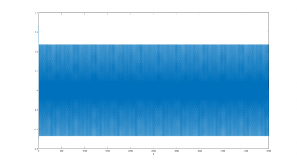
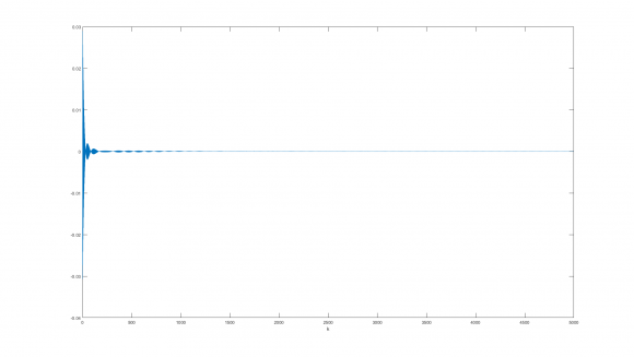
Then I use the following MATLAB code to do zero-input limit cycle test

%%%%%%%%%%%%%%%%%%%%%%%%%%%%%%%%%%%%%%%%%%%%%%%%%%%%%%

L=16;%word length

for k=0:4999

%% initial value %%

if k==0

x=fi([0.1;0.1;0.1;0.1;0.1;0.1],1,L); %initial state

u=fi(0,1,L); %input

else

x(1:6,k+1)=fi(A,1,L)*x(1:6,k)+fi(B,1,L)*u;% state equation

y(k)=fi(C,1,L)*x(1:6,k)+fi(D,1,L)*u;% output

end

end

figure;

plot(0:4998, y,'-'); %plot the output response

xlabel('k');

%%%%%%%%%%%%%%%%%%%%%%%%%%%%%%%%%%%%%%%%%%%%%%%%%%%%%%%

The output of the canonical form filter

The output of the developed filter

I am not familiar with DSP processors. Is state-space model suitable for implementing in a DSP? 

well, i don't have the fixed=point toolbox, but if you're plagued with limit cycles due to round-to-nearest quantization, my suggestion is that you use a technique colloquially called "fraction saving" but could also be called "noise-shaping with a zero at z=1".

It works like this:  

1. Always round down (toward -infinity).  This is the same as dropping bits to the right of the quantization point of the larger word being shortened to a smaller word.

2. Whatever bits are dropped, save those bits in a state.

3. In the following sample, before quantization (step 1.) add those bits that you dropped, zero extended on the left, to the larger word immediately before the quantization operation of step 1.

This will give you infinite signal-to-noise ration at the frequency of 0 Hz, and you pay for it with increased quantization noise at Nyquist.

That's the way I got rid of limit cycles due to fixed-point arithmetic and quantization.

That's a new one for me.  I'm trying to understand why this works.

From frequency-domain point of view, the new filter structure is composed of coupled-form second order sections (or biquad) in parallel form and is with appropriate scaling factor to minimize L_2 sensitivity (or zero sensitivity) as well.

Indeed, the developed filter was derived by some mathematical theorems (mainly linear algebra and matrix calculus). 

The key reason to reduce pole sensitivity and limit cycles is the so-called normal-form state transition matrix of the state-space model.

A normal-form filter is with globally minimal pole-sensitivity and limit-cycle-free property.

This property was first investigated by Mullis and Roberts [1] AND BARNES and FAM [2].

However, these works did not focus on how synthesizing a high order normal-form filter.

In 1997, Li [3] proposed an interesting method to synthesize a filter with minimal pole-zero sensitivity measure. In this paper, a normal-form state transition matrix can be obtained by a closed-form solution. However, the synthesized normal-form state transition matrix is fully parameterized ((n+1)^2 multiplications are needed per output sample), and repeated zeros cannot be allowed. In addition, except the normal-form state transformation matrix, the entire filter parameters are synthesized by the gradient descent searching algorithm.

To date, a computationally efficient high-order normal-form filter with minimal zero/L_2 sensitivity synthesis is still an open problem.

This is the main motivation that I want to develop the new method to synthesize the filter structure.

The developed result is still under review by an IEEE Transaction.

I am an academic researcher, not an engineer.

I once discussed with my colleague and he told me that state-space model is not popular in signal processing society.  

So I want to have some discussions with the people who are familiar with DSP/signal processing engineering, to ensure that my research is helpful for real applications.

Finally, please forgive me if my English usage is not appropriate since it is not my native language.

[1] C. T. Mullis and R. A. Roberts, “Synthesis of minimum roundoff noise

fixed point digital filters.” IEEE Trans. Circuits Syst., vol. 23, no. 9, pp. 551–562, 1976.

[2] C.Barnes and A. Fam, “Minimum norm recursive digital filters that are free of overflow limit cycles,” IEEE Trans. Circuits Syst., vol. 24, no. 10, pp. 569–574, 1977.

[3] G.Li, “On pole and zero sensitivity of linear systems.,” IEEE Trans. Circuits Syst. I Fundam. Theory Appl., vol. 44, no. 7, pp. 583–590, 1997.