


Converting Signal Flow Graphs to State-Space Form by Hand
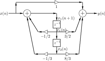
The procedure of the previous section quickly converts any transfer function to state-space form (specifically, controller canonical form). When the starting point is instead a signal flow graph, it is usually easier to go directly to state-space form by labeling each delay-element output as a state variable and writing out the state-space equations by inspection of the flow graph.
For the example of the previous section, suppose we are given
Eq.![]() (G.14) in direct-form II (DF-II), as shown in
Fig.G.1. It is important that the filter representation be
canonical with respect to delay, i.e., that the number of
delay elements equals the order of the filter. Then the third step
(writing down controller canonical form by inspection) may replaced by the
following more general procedure:
(G.14) in direct-form II (DF-II), as shown in
Fig.G.1. It is important that the filter representation be
canonical with respect to delay, i.e., that the number of
delay elements equals the order of the filter. Then the third step
(writing down controller canonical form by inspection) may replaced by the
following more general procedure:
- Assign a state variable to the output of each delay element (indicated in Fig.G.1).
- Write down the state-space representation by inspection of the flow graph.
 |
The state-space description of the difference equation in
Eq.![]() (G.7) is given by Eq.
(G.7) is given by Eq.![]() (G.16).
We see that controller canonical form follows immediately from the
direct-form-II digital filter realization, which is fundamentally an
all-pole filter followed by an all-zero (FIR) filter (see
§9.1.2). By starting instead from the
transposed direct-form-II (TDF-II) structure, the
observer canonical form is obtained [28, p.
87]. This is because the zeros effectively precede the
poles in a TDF-II realization, so that they may introduce nulls in the
input spectrum, but they cannot cancel output from the poles (e.g.,
from initial conditions). Since the other two digital-filter direct
forms (DF-I and TDF-I--see Chapter 9 for details) are not canonical
with respect to delay, they are not used as a basis for deriving
state-space models.
(G.16).
We see that controller canonical form follows immediately from the
direct-form-II digital filter realization, which is fundamentally an
all-pole filter followed by an all-zero (FIR) filter (see
§9.1.2). By starting instead from the
transposed direct-form-II (TDF-II) structure, the
observer canonical form is obtained [28, p.
87]. This is because the zeros effectively precede the
poles in a TDF-II realization, so that they may introduce nulls in the
input spectrum, but they cannot cancel output from the poles (e.g.,
from initial conditions). Since the other two digital-filter direct
forms (DF-I and TDF-I--see Chapter 9 for details) are not canonical
with respect to delay, they are not used as a basis for deriving
state-space models.
Next Section:
Controllability and Observability
Previous Section:
Converting to State-Space Form by Hand


