


Converting to State-Space Form by Hand
Converting a digital filter to state-space form is easy because there are various ``canonical forms'' for state-space models which can be written by inspection given the strictly proper transfer-function coefficients.
The canonical forms useful for transfer-function to state-space conversion are controller canonical form (also called control or controllable canonical form) and observer canonical form (or observable canonical form) [28, p. 80], [37]. These names come from the field of control theory [28] which is concerned with designing feedback laws to control the dynamics of real-world physical systems. State-space models are used extensively in the control field to model physical systems.
The name ``controller canonical form'' reflects the fact that the
input signal can ``drive'' all modes (poles) of the system. In the
language of control theory, we may say that all of the system poles
are controllable from the input
![]() . In observer canonical form, all modes are guaranteed to be
observable. Controllability and observability of a state-space
model are discussed further in §G.7.3 below.
. In observer canonical form, all modes are guaranteed to be
observable. Controllability and observability of a state-space
model are discussed further in §G.7.3 below.
The following procedure converts any causal LTI digital filter into state-space form:
- Determine the filter transfer function
 .
.
- If
 is not strictly proper (
 ),
``pull out'' the delay-free path
to obtain a feed-through gain
),
``pull out'' the delay-free path
to obtain a feed-through gain  in parallel with a strictly
proper transfer function.
in parallel with a strictly
proper transfer function.
- Write down the state-space representation by inspection using controller canonical form for the strictly proper transfer function. (Or use the matlab function tf2ss.)
We now elaborate on these steps for the general case:
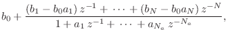
- The general causal IIR filter
has transfer function
- By convention, state-space descriptions handle any delay-free
path from input to output via the direct-path coefficient
 in
Eq.
in
Eq. (G.1). This is natural because the delay-free path does not
affect the state of the system.
(G.1). This is natural because the delay-free path does not
affect the state of the system.
A causal filter contains a delay-free path if its impulse response
 is nonzero at time zero, i.e., if
 .G.5 In such cases, we must ``pull out'' the
delay-free path in order to implement it in parallel, setting
.G.5 In such cases, we must ``pull out'' the
delay-free path in order to implement it in parallel, setting
 in the state-space model.
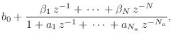
In our example, one step of long division yields
where , with
 for
for  , and
, and
 for
for  .
.
- The controller canonical form is then easily written as follows:
An alternate controller canonical form is obtained by applying the similarity transformation (see §G.8 below) which simply reverses the order of the state variables. Any permutation of the state variables would similarly yield a controllable form. The transpose of a controllable form is an observable form.
![\begin{displaymath}\left[
\begin{array}{ccccc}
-a_1 & -a_2 & \cdots & -a_{N-1} &...
...\ [2pt] 0 \\ [2pt] \vdots\\ [2pt] 0\end{array}\right]
\nonumber\end{displaymath}](http://www.dsprelated.com/josimages_new/filters/img2121.png)
One might worry that choosing controller canonical form may result in
unobservable modes. However, this will not happen if ![]() and
and
![]() have no common factors. In other words, if there are no
pole-zero cancellations in the transfer function
have no common factors. In other words, if there are no
pole-zero cancellations in the transfer function
![]() ,
then either controller or observer canonical form will yield a
controllable and observable state-space model.
,
then either controller or observer canonical form will yield a
controllable and observable state-space model.
We now illustrate these steps using the example of Eq.![]() (G.7):
(G.7):
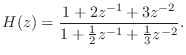
- The transfer function can be written, by inspection, as
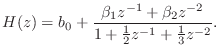
- We need to convert Eq.(G.13) to the form
Obtaining a common denominator and equating numerator coefficients with Eq.(G.13) yields
The same result is obtained using long division (or synthetic division). - Finally, the controller canonical form is given by
![$\displaystyle \left[\begin{array}{cc} -\frac{1}{2} & -\frac{1}{3} \\ [2pt] 1 & 0 \end{array}\right]$](http://www.dsprelated.com/josimages_new/filters/img2132.png)
Next Section:
Converting Signal Flow Graphs to State-Space Form by Hand
Previous Section:
Example State Space Filter Transfer Function


