


Implementation Structures for Recursive Digital Filters
This chapter introduces the four direct-form filter implementations, and discusses implementation of filters as parallel or series combinations of smaller filter sections. A careful study of filter forms can be important when numerical issues arise, such as when implementing a digital filter in a fixed-point processor. (The least expensive ``DSP chips'' use fixed-point numerical processing, sometimes with only a 16-bit word length in low-cost audio applications.) For implementations in floating-point arithmetic, especially at 32-bit word-lengths or greater, the choice of filter implementation structure is usually not critical. In matlab software, for example, one rarely uses anything but the filter function, which is implemented in double-precision floating point (typically 64 bits at the time of this writing, and more bits internally in the floating-point unit).
The Four Direct Forms
Direct-Form I
As mentioned in §5.5,
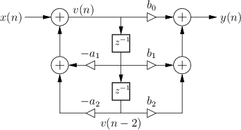
the difference equation
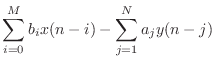 |
(10.1) |
specifies the Direct-Form I (DF-I) implementation of a digital filter [60]. The DF-I signal flow graph for the second-order case is shown in Fig.9.1.
The DF-I structure has the following properties:
- It can be regarded as a two-zero filter section followed in series
by a two-pole filter section.
- In most fixed-point arithmetic schemes (such as two's complement,
the most commonly used
[84]10.1)
there is no possibility of internal filter overflow. That is,
since there is fundamentally only one summation point in the filter,
and since fixed-point overflow naturally ``wraps around'' from the
largest positive to the largest negative number and vice versa, then
as long as the final result
 is ``in range'', overflow is
avoided, even when there is overflow of intermediate results in the sum
(see below for an example). This is an important, valuable, and
unusual property of the DF-I filter structure.
is ``in range'', overflow is
avoided, even when there is overflow of intermediate results in the sum
(see below for an example). This is an important, valuable, and
unusual property of the DF-I filter structure.
- There are twice as many delays as are necessary. As a result,
the DF-I structure is not canonical with respect to delay. In
general, it is always possible to implement an
 th-order filter
using only delay elements.
th-order filter
using only delay elements.
- As is the case with all direct-form filter structures
(those which have coefficients given by the transfer-function coefficients),
the filter poles and zeros can be very sensitive to round-off errors
in the filter coefficients. This is usually not a problem for a
simple second-order section, such as in Fig.9.1, but it can
become a problem for higher order direct-form filters. This is the
same numerical sensitivity that polynomial roots have with respect to
polynomial-coefficient round-off. As is well known, the sensitivity
tends to be larger when the roots are clustered closely together, as
opposed to being well spread out in the complex plane
[18, p. 246]. To minimize this sensitivity, it is common to
factor filter transfer functions into series and/or parallel second-order
sections, as discussed in §9.2 below.
It is a very useful property of the direct-form I implementation that it cannot overflow internally in two's complement fixed-point arithmetic: As long as the output signal is in range, the filter will be free of numerical overflow. Most IIR filter implementations do not have this property. While DF-I is immune to internal overflow, it should not be concluded that it is always the best choice of implementation. Other forms to consider include parallel and series second-order sections (§9.2 below), and normalized ladder forms [32,48,86].10.2Also, we'll see that the transposed direct-form II (Fig.9.4 below) is a strong contender as well.
Two's Complement Wrap-Around
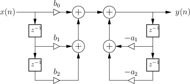
In this section, we give an example showing how temporary overflow in two's complement fixed-point causes no ill effects.
In 3-bit signed fixed-point arithmetic, the available numbers are as shown in Table 9.1.
|
Let's perform the sum ![]() , which gives a temporary overflow
(
, which gives a temporary overflow
(![]() , which wraps around to
, which wraps around to ![]() ), but a final result (
), but a final result (![]() ) which
is in the allowed range
) which
is in the allowed range ![]() :10.3
:10.3
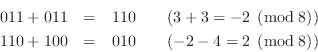
Now let's do ![]() in three-bit two's complement:
in three-bit two's complement:
In both examples, the intermediate result overflows, but the final result is correct. Another way to state what happened is that a positive wrap-around in the first addition is canceled by a negative wrap-around in the second addition.
Direct Form II
The signal flow graph for the Direct-Form-II (DF-II) realization of the second-order IIR filter section is shown in Fig.9.2.
The difference equation for the second-order DF-II structure can be written as
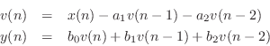
which can be interpreted as a two-pole filter followed in series by a two-zero filter. This contrasts with the DF-I structure of the previous section (diagrammed in Fig.9.1) in which the two-zero FIR section precedes the two-pole recursive section in series. Since LTI filters in series commute (§6.7), we may reverse this ordering and implement an all-pole filter followed by an FIR filter in series. In other words, the zeros may come first, followed by the poles, without changing the transfer function. When this is done, it is easy to see that the delay elements in the two filter sections contain the same numbers (see Fig.5.1). As a result, a single delay line can be shared between the all-pole and all-zero (FIR) sections. This new combined structure is called ``direct form II'' [60, p. 153-155]. The second-order case is shown in Fig.9.2. It specifies exactly the same digital filter as shown in Fig.9.1 in the case of infinite-precision numerical computations.
In summary, the DF-II structure has the following properties:
- It can be regarded as a two-pole filter section followed by a two-zero
filter section.
- It is canonical with respect to delay. This happens because
delay elements associated with the two-pole and two-zero sections are
shared.
- In fixed-point arithmetic, overflow can
occur at the delay-line input (output
of the leftmost summer in Fig.9.2), unlike in the DF-I
implementation.
- As with all direct-form filter structures, the poles
and zeros are sensitive to round-off errors in the coefficients
 and
and  , especially for high transfer-function orders. Lower
sensitivity is obtained using series low-order sections (e.g., second
order), or by using ladder or lattice filter structures
[86].
, especially for high transfer-function orders. Lower
sensitivity is obtained using series low-order sections (e.g., second
order), or by using ladder or lattice filter structures
[86].
More about Potential Internal Overflow of DF-II
Since the poles come first in the DF-II realization of an IIR filter,
the signal entering the state delay-line (see Fig.9.2) typically
requires a larger dynamic range than the output signal ![]() . In
other words, it is common for the feedback portion of a DF-II IIR
filter to provide a large signal boost which is then
compensated by attenuation in the feedforward portion (the
zeros). As a result, if the input dynamic range is to remain
unrestricted, the two delay elements may need to be implemented with
high-order guard bits to accommodate an extended dynamic range.
If the number of bits in the delay elements is doubled (which still
does not guarantee impossibility of internal overflow), the benefit of
halving the number of delays relative to the DF-I structure is
approximately canceled. In other words, the DF-II structure, which is
canonical with respect to delay, may require just as much or more
memory as the DF-I structure, even though the DF-I uses twice as many
addressable delay elements for the filter state memory.
. In
other words, it is common for the feedback portion of a DF-II IIR
filter to provide a large signal boost which is then
compensated by attenuation in the feedforward portion (the
zeros). As a result, if the input dynamic range is to remain
unrestricted, the two delay elements may need to be implemented with
high-order guard bits to accommodate an extended dynamic range.
If the number of bits in the delay elements is doubled (which still
does not guarantee impossibility of internal overflow), the benefit of
halving the number of delays relative to the DF-I structure is
approximately canceled. In other words, the DF-II structure, which is
canonical with respect to delay, may require just as much or more
memory as the DF-I structure, even though the DF-I uses twice as many
addressable delay elements for the filter state memory.
Transposed Direct-Forms
The remaining two direct forms are obtained by formally transposing direct-forms I and II [60, p. 155]. Filter transposition may also be called flow graph reversal, and transposing a Single-Input, Single-Output (SISO) filter does not alter its transfer function. This fact can be derived as a consequence of Mason's gain formula for signal flow graphs [49,50] or Tellegen's theorem (which implies that an LTI signal flow graph is interreciprocal with its transpose) [60, pp. 176-177]. Transposition of filters in state-space form is discussed in §G.5.
The transpose of a SISO digital filter is quite straightforward to find: Reverse the direction of all signal paths, and make obviously necessary accommodations. ``Obviously necessary accommodations'' include changing signal branch-points to summers, and summers to branch-points. Also, after this operation, the input signal, normally drawn on the left of the signal flow graph, will be on the right, and the output on the left. To renormalize the layout, the whole diagram is usually left-right flipped.
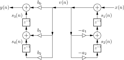
Figure 9.3 shows the Transposed-Direct-Form-I (TDF-I) structure for the general second-order IIR digital filter, and Fig.9.4 shows the Transposed-Direct-Form-II (TDF-II) structure. To facilitate comparison of the transposed with the original, the inputs and output signals remain ``switched'', so that signals generally flow right-to-left instead of the usual left-to-right. (Exercise: Derive forms TDF-I/II by transposing the DF-I/II structures shown in Figures 9.1 and 9.2.)
 |
 |
Numerical Robustness of TDF-II
An advantage of the transposed direct-form II structure (depicted in
Fig.9.4) is that the zeros effectively precede the poles in
series order. As mentioned above, in many digital filters design, the
poles by themselves give a large gain at some frequencies, and the
zeros often provide compensating attenuation. This is especially true
of filters with sharp transitions in their frequency response, such as
the elliptic-function-filter example on page ![]() ; in such
filters, the sharp transitions are achieved using near pole-zero
cancellations close to the unit circle in the
; in such
filters, the sharp transitions are achieved using near pole-zero
cancellations close to the unit circle in the ![]() plane.10.4
plane.10.4
Series and Parallel Filter Sections
In many situations it is better to implement a digital filter ![]() in terms of first- and/or second-order elementary sections,
either in series or in parallel. In particular, such an
implementation may have numerical advantages. In the time-varying
case, it is easier to control fundamental parameters of small
sections, such as pole frequencies, by means of coefficient
variations.
in terms of first- and/or second-order elementary sections,
either in series or in parallel. In particular, such an
implementation may have numerical advantages. In the time-varying
case, it is easier to control fundamental parameters of small
sections, such as pole frequencies, by means of coefficient
variations.
Series Second-Order Sections
For many filter types, such as lowpass, highpass, and bandpass filters, a good choice of implementation structure is often series second-order sections. In fixed-point applications, the ordering of the sections can be important.
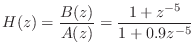
The matlab function tf2sos10.5 converts from ``transfer function form'',
![]() , to series ``second-order-section'' form.
For example, the line
, to series ``second-order-section'' form.
For example, the line
BAMatrix = tf2sos(B,A);converts the real filter specified by polynomial vectors B and A to a series of second-order sections (biquads) specified by the rows of BAMatrix. Each row of BAMatrix is of the form
function [sos,g] = tf2sos(B,A)
[z,p,g]=tf2zp(B(:)',A(:)'); % Direct form to (zeros,poles,gain)
sos=zp2sos(z,p,g); % (z,p,g) to series second-order sections
Matlab Example
The following matlab example expands the filter
B=[1 0 0 0 0 1];
A=[1 0 0 0 0 .9];
[sos,g] = tf2sos(B,A)
sos =
   1.00000   0.61803   1.00000   1.00000   0.60515   0.95873
   1.00000  -1.61803   1.00000   1.00000  -1.58430   0.95873
   1.00000   1.00000  -0.00000   1.00000   0.97915  -0.00000

g = 1
The g parameter is an input (or output) scale factor; for this filter, it was not needed. Thus, in this example we obtained the following filter factorization:
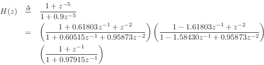
Note that the first two sections are second-order, while the third is first-order (when coefficients are rounded to five digits of precision after the decimal point).
In addition to tf2sos, tf2zp, and zp2sos discussed above, there are also functions sos2zp and sos2tf, which do the obvious conversion in both Matlab and Octave.10.6 The sos2tf function can be used to check that the second-order factorization is accurate:
% Numerically challenging "clustered roots" example:
[B,A] = zp2tf(ones(10,1),0.9*ones(10,1),1);
[sos,g] = tf2sos(B,A);
[Bh,Ah] = sos2tf(sos,g);
format long;
disp(sprintf('Relative L2 numerator error: %g',...
	norm(Bh-B)/norm(B)));
% Relative L2 numerator error: 1.26558e-15
disp(sprintf('Relative L2 denominator error: %g',...
	norm(Ah-A)/norm(A)));
% Relative L2 denominator error: 1.65594e-15
Thus, in this test, the original direct-form filter is compared with
one created from the second-order sections. Such checking should be
done for high-order filters, or filters having many poles and/or zeros
close together, because the polynomial factorization used to find the
poles and zeros can fail numerically. Moreover, the stability of the
factors should be checked individually.
Parallel First and/or Second-Order Sections
Instead of breaking up a filter into a series of second-order
sections, as discussed in the previous section, we can break the
filter up into a parallel sum of first and/or second-order
sections. Parallel sections are based directly on the partial
fraction expansion (PFE) of the filter transfer function discussed in
§6.8. As discussed in §6.8.3, there is additionally an
FIR part when the order of the transfer-function denominator
does not exceed that of the numerator (i.e., when the transfer function
is not strictly proper). The most general case of a PFE, valid
for any finite-order transfer function, was given by Eq.![]() (6.19),
repeated here for convenience:
(6.19),
repeated here for convenience:
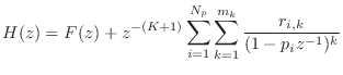
where
The FIR part ![]() is typically realized as a tapped delay line, as
shown in Fig.5.5.
is typically realized as a tapped delay line, as
shown in Fig.5.5.
First-Order Complex Resonators
For distinct poles, the recursive terms in the complete partial
fraction expansion of Eq.![]() (9.2) can be realized as a parallel sum
of complex one-pole filter
sections, thereby producing a parallel complex resonator filter
bank. Complex resonators are efficient for processing complex input
signals, and they are especially easy to work with. Note that a
complex resonator bank is similarly obtained by implementing a
diagonalized state-space model [Eq.
(9.2) can be realized as a parallel sum
of complex one-pole filter
sections, thereby producing a parallel complex resonator filter
bank. Complex resonators are efficient for processing complex input
signals, and they are especially easy to work with. Note that a
complex resonator bank is similarly obtained by implementing a
diagonalized state-space model [Eq.![]() (G.22)].
(G.22)].
Real Second-Order Sections
In practice, however, signals are typically real-valued functions of
time. As a result, for real filters (§5.1),
it is typically more efficient computationally to combine
complex-conjugate one-pole sections together to form real second-order
sections (two poles and one zero each, in general). This process was
discussed in §6.8.1, and the resulting transfer function of
each second-order section becomes
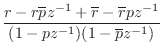
where
When the two poles of a real second-order section are complex, they
form a complex-conjugate pair, i.e., they are located at
![]() in the
in the ![]() plane, where
plane, where ![]() is the modulus of either
pole, and
is the modulus of either
pole, and ![]() is the angle of either pole. In this case, the
``resonance-tuning coefficient'' in Eq.
is the angle of either pole. In this case, the
``resonance-tuning coefficient'' in Eq.![]() (9.3) can be expressed as
(9.3) can be expressed as
Figures 3.25 and 3.26 (p. ![]() ) illustrate filter realizations
consisting of one first-order and two second-order filter sections in
parallel.
) illustrate filter realizations
consisting of one first-order and two second-order filter sections in
parallel.
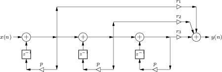
Implementation of Repeated Poles
Fig.9.5 illustrates an efficient implementation of terms due to a repeated pole with multiplicity three, contributing the additive terms
Formant Filtering Example
In speech synthesis [27,39], digital filters are often used to simulate formant filtering by the vocal tract. It is well known [23] that the different vowel sounds of speech can be simulated by passing a ``buzz source'' through a only two or three formant filters. As a result, speech is fully intelligible through the telephone bandwidth (nominally only 200-3200 Hz).
A formant is a resonance in the voice spectrum. A
single formant may thus be modeled using one biquad
(second-order filter section). For example, in the vowel ![]() as in
``father,'' the first three formant center-frequencies have been
measured near 700, 1220, and 2600 Hz, with half-power
bandwidths10.7 130, 70, and 160 Hz [40].
as in
``father,'' the first three formant center-frequencies have been
measured near 700, 1220, and 2600 Hz, with half-power
bandwidths10.7 130, 70, and 160 Hz [40].
In principle, the formant filter sections are in series, as can be found by deriving the transfer function of an acoustic tube [48]. As a consequence, the vocal-tract transfer function is an all-pole filter (provided that the nasal tract is closed off or negligible). As a result, there is no need to specify gains for the formant resonators--only center-frequency and bandwidth are necessary to specify each formant, leaving only an overall scale factor unspecified in a cascade (series) formant filter bank.
Numerically, however, it makes more sense to implement disjoint resonances in parallel rather than in series.10.8 This is because when one formant filter is resonating, the others will be attenuating, so that to achieve a particular peak-gain at resonance, the resonating filter must overcome all combined attenuations as well as applying its own gain. In fixed-point arithmetic, this can result in large quantization-noise gains, especially for the last resonator in the chain. As a result of these considerations, our example will implement the formant sections in parallel. This means we must find the appropriate biquad numerators so that when added together, the overall transfer-function numerator is a constant. This will be accomplished using the partial fraction expansion (§6.8).10.9
The matlab below illustrates the construction of a parallel formant
filter bank for simulating the vowel ![]() . For completeness, it is
used to filter a bandlimited impulse train, in order to synthesize the
vowel sound.
. For completeness, it is
used to filter a bandlimited impulse train, in order to synthesize the
vowel sound.
F =  [700, 1220, 2600]; % Formant frequencies (Hz)
BW = [130,  70,  160];  % Formant bandwidths (Hz)
fs = 8192;              % Sampling rate (Hz)

nsecs = length(F);
R = exp(-pi*BW/fs);     % Pole radii
theta = 2*pi*F/fs;      % Pole angles
poles = R .* exp(j*theta); % Complex poles
B = 1;  A = real(poly([poles,conj(poles)]));
% freqz(B,A); % View frequency response:

% Convert to parallel complex one-poles (PFE):
[r,p,f] = residuez(B,A);
As = zeros(nsecs,3);
Bs = zeros(nsecs,3);
% complex-conjugate pairs are adjacent in r and p:
for i=1:2:2*nsecs
    k = 1+(i-1)/2;
    Bs(k,:) = [r(i)+r(i+1),  -(r(i)*p(i+1)+r(i+1)*p(i)), 0];
    As(k,:) = [1, -(p(i)+p(i+1)), p(i)*p(i+1)];
end
sos = [Bs,As]; % standard second-order-section form
iperr = norm(imag(sos))/norm(sos); % make sure sos is ~real
disp(sprintf('||imag(sos)||/||sos|| = %g',iperr)); % 1.6e-16
sos = real(sos) % and make it exactly real

% Reconstruct original numerator and denominator as a check:
[Bh,Ah] = psos2tf(sos); % parallel sos to transfer function
% psos2tf appears in the matlab-utilities appendix
disp(sprintf('||A-Ah|| = %g',norm(A-Ah))); % 5.77423e-15
% Bh has trailing epsilons, so we'll zero-pad B:
disp(sprintf('||B-Bh|| = %g',...
             norm([B,zeros(1,length(Bh)-length(B))] - Bh)));
% 1.25116e-15

% Plot overlay and sum of all three
% resonator amplitude responses:
nfft=512;
H = zeros(nsecs+1,nfft);
for i=1:nsecs
  [Hiw,w] = freqz(Bs(i,:),As(i,:));
  H(1+i,:) = Hiw(:).';
end
H(1,:) = sum(H(2:nsecs+1,:));
ttl = 'Amplitude Response';
xlab = 'Frequency (Hz)';
ylab = 'Magnitude (dB)';
sym = '';
lgnd = {'sum','sec 1','sec 2', 'sec 3'};
np=nfft/2; % Only plot for positive frequencies
wp = w(1:np); Hp=H(:,1:np);
figure(1); clf;
myplot(wp,20*log10(abs(Hp)),sym,ttl,xlab,ylab,1,lgnd);
disp('PAUSING'); pause;
saveplot('../eps/lpcexovl.eps');

% Now synthesize the vowel [a]:
nsamps = 256;
f0 = 200; % Pitch in Hz
w0T = 2*pi*f0/fs; % radians per sample

nharm = floor((fs/2)/f0); % number of harmonics
sig = zeros(1,nsamps);
n = 0:(nsamps-1);
% Synthesize bandlimited impulse train
for i=1:nharm,
    sig = sig + cos(i*w0T*n);
end;
sig = sig/max(sig);
speech = filter(1,A,sig);
soundsc([sig,speech]); % hear buzz, then 'ah'
Notes:
- The sampling rate was chosen to
be
 Hz because that is the default Matlab sampling rate,
and because that is a typical value used for ``telephone quality''
speech synthesis.
Hz because that is the default Matlab sampling rate,
and because that is a typical value used for ``telephone quality''
speech synthesis.
- The psos2tf utility is listed in §J.7.
- The overlay of the amplitude responses are shown in Fig.9.6.
![\includegraphics[width=\twidth]{eps/lpcexovl}](http://www.dsprelated.com/josimages_new/filters/img1163.png)
Butterworth Lowpass Filter Example
This example illustrates the design of a 5th-order Butterworth lowpass filter, implementing it using second-order sections. Since all three sections contribute to the same passband and stopband, it is numerically advisable to choose a series second-order-section implementation, so that their passbands and stopbands will multiply together instead of add.
fc = 1000; % Cut-off frequency (Hz)
fs = 8192; % Sampling rate (Hz)
order = 5; % Filter order
[B,A] = butter(order,2*fc/fs); % [0:pi] maps to [0:1] here
[sos,g] = tf2sos(B,A)
% sos =
%  1.00000  2.00080   1.00080  1.00000  -0.92223  0.28087
%  1.00000  1.99791   0.99791  1.00000  -1.18573  0.64684
%  1.00000  1.00129  -0.00000  1.00000  -0.42504  0.00000
%
% g = 0.0029714
%
% Compute and display the amplitude response
Bs = sos(:,1:3); % Section numerator polynomials
As = sos(:,4:6); % Section denominator polynomials
[nsec,temp] = size(sos);
nsamps = 256; % Number of impulse-response samples
% Note use of input scale-factor g here:
x = g*[1,zeros(1,nsamps-1)]; % SCALED impulse signal
for i=1:nsec
  x = filter(Bs(i,:),As(i,:),x); % Series sections
end
%
%plot(x); % Plot impulse response to make sure
          % it has decayed to zero (numerically)
%
% Plot amplitude response
% (in Octave - Matlab slightly different):
figure(2);
X=fft(x); % sampled frequency response
f = [0:nsamps-1]*fs/nsamps; grid('on');
axis([0 fs/2 -100 5]); legend('off');
plot(f(1:nsamps/2),20*log10(X(1:nsamps/2)));
The final plot appears in Fig.9.7. A Matlab function for frequency response plots is given in §J.4. (Of course, one can also use freqz in either Matlab or Octave, but that function uses subplots which are not easily printable in Octave.)
Note that the Matlab Signal Processing Toolbox has a function called sosfilt so that ``y=sosfilt(sos,x)'' will implement an array of second-order sections without having to unpack them first as in the example above.
![\includegraphics[width=0.8\twidth]{eps/buttlpex}](http://www.dsprelated.com/josimages_new/filters/img1164.png) |
Summary of Series/Parallel Filter Sections
In summary, we noted above the following general guidelines regarding series vs. parallel elementary-section implementations:
- Series sections are preferred when all sections contribute to the same passband, such as in a lowpass, highpass, bandpass, or bandstop filter.
- Parallel sections are usually preferred when the sections have disjoint passbands, such as a formant filter bank used in voice models. Another example would be the phase vocoder filter bank [21].
Pole-Zero Analysis Problems
See http://ccrma.stanford.edu/~jos/filtersp/Pole_Zero_Analysis_Problems.html.
Next Section:
Filters Preserving Phase
Previous Section:
Pole-Zero Analysis


