DSPRelated.com
Free Books

Parallel Case

Figure 6.2: Parallel combination of transfer functions $ H_1(z)$ and $ H_2(z)$, yielding $ H(z)=H_1(z)+H_2(z)$.
\begin{figure}\input fig/parallel.pstex_t
\end{figure}

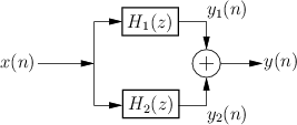
Figure 6.2 illustrates the parallel combination of two filters. The filters $ H_1(z)$ and $ H_2(z)$ are driven by the same input signal $ x(n)$, and their respective outputs $ y_1(n)$ and $ y_2(n)$ are summed. The transfer function of the parallel combination is therefore

$\displaystyle H(z) \isdefs \frac{Y(z)}{X(z)} \eqsp \frac{Y_1(z) + Y_2(z)}{X(z)}
\eqsp \frac{Y_1(z)}{X(z)} + \frac{Y_2(z)}{X(z)} \isdefs H_1(z)+H_2(z).
$

where we needed only linearity of the z transform to have that $ {\cal Z}\{y_1+y_2\} = {\cal Z}\{y_1\}+{\cal Z}\{y_2\}$.

Series Combination is Commutative

Since multiplication of complex numbers is commutative, we have

$\displaystyle H_1(z)H_2(z)=H_2(z)H_1(z),
$

which implies that any ordering of filters in series results in the same overall transfer function. Note, however, that the numerical performance of the overall filter is usually affected by the ordering of filter stages in a series combination [103]. Chapter 9 further considers numerical performance of filter implementation structures.

By the convolution theorem for z transforms, commutativity of a product of transfer functions implies that convolution is commutative:

$\displaystyle h_1 \ast h_2
\;\leftrightarrow\;
H_1\cdot H_2
\;=\;
H_2\cdot H_1
\;\leftrightarrow\;
h_2 \ast h_1
$


Next Section:
Example
Previous Section:
Series Case