DSPRelated.com
Free Books

RLC Filter Analysis

Referring now to Fig.E.2, let's perform an impedance analysis of that RLC network.

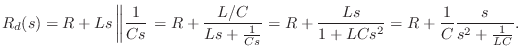
Driving Point Impedance

By inspection, we can write
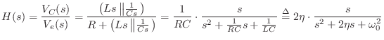
$\displaystyle R_d(s) = R + Ls \left\Vert \frac{1}{Cs}\right.
= R +\frac{L/C}{L...
...}{Cs}}
= R + \frac{Ls}{1+LCs^2} = R + \frac{1}{C}
\frac{s}{s^2+\frac{1}{LC}}.
$

where $ \Vert$ denotes ``in parallel with,'' and we used the general formula, memorized by any electrical engineering student,

$\displaystyle \zbox {R_1 \Vert R_2 = \frac{R_1 R_2}{R_1 + R_2}.}
$

That is, the impedance of the parallel combination of impedances $ R_1$ and $ R_2$ is given by the product divided by the sum of the impedances.


Transfer Function

The transfer function in this example can similarly be found using voltage divider rule:
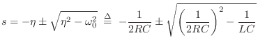
$\displaystyle H(s) = \frac{V_C(s)}{V_e(s)}
= \frac{\left(Ls\left\Vert\frac{1}{...
...1}{RC} s + \frac{1}{LC}}
\isdef 2\eta\cdot\frac{s}{s^2 + 2\eta s + \omega_0^2}
$


Poles and Zeros

From the quadratic formula, the two poles are located at
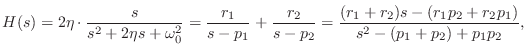
$\displaystyle s =
-\eta \pm \sqrt{\eta^2 - \omega_0^2}
\;\isdef \;
-\frac{1}{2RC} \pm \sqrt{\left(\frac{1}{2RC}\right)^2 - \frac{1}{LC}}
$

and there is a zero at $ s=0$ and another at $ s=\infty$. If the damping $ R$ is sufficienly small so that $ \eta^2 < \omega_0^2$, then the poles form a complex-conjugate pair:

$\displaystyle s = -\eta \pm j\sqrt{\omega_0^2 - \eta^2}
$

Since $ \eta = 1/(2RC) > 0$, the poles are always in the left-half plane, and hence the analog RLC filter is always stable. When the damping is zero, the poles go to the $ j\omega$ axis:

$\displaystyle s = \pm j\omega_0
$


Impulse Response

The impulse response is again the inverse Laplace transform of the transfer function. Expanding $ H(s)$ into a sum of complex one-pole sections,

$\displaystyle H(s) = 2\eta\cdot\frac{s}{s^2 + 2\eta s + \omega_0^2}
= \frac{r_...
...r_2}{s-p_2}
= \frac{(r_1+r_2)s - (r_1p_2 + r_2p_1)}{s^2-(p_1 + p_2) + p_1p_2},
$

where $ p_{1,2}\isdef -\eta \pm \sqrt{\eta^2 - \omega_0^2}$. Equating numerator coefficients gives

\begin{eqnarray*}
r_1+r_2 &=& 2\eta \;\mathrel{=}\; \frac{1}{RC}\\
r_1p_2 + r_2p_1 &=& 0.
\end{eqnarray*}

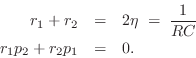
This pair of equations in two unknowns may be solved for $ r_1$ and $ r_2$. The impulse response is then

$\displaystyle h(t) = r_1 e^{p_1 t} u(t) + r_2 e^{p_2 t} u(t).
$


Next Section:
Relating Pole Radius to Bandwidth
Previous Section:
RC Filter Analysis