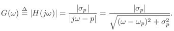
Consider the continuous-time complex one-pole
resonator with  -plane transfer function
where

is the
Laplace-transform variable, and

is the single complex pole. The numerator scaling
has been set to

so that the
frequency response is normalized to
unity gain at resonance:
The
amplitude response at all frequencies is given by
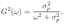
Without loss of generality, we may set

, since changing

merely translates the amplitude response with respect to

.
(We could alternatively define the translated frequency variable

to get the same simplification.) The squared amplitude response is now
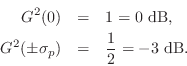
Note that
This shows that the 3-dB bandwidth of the resonator in radians
per second is
 , or twice the absolute value of the real
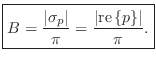
part of the pole. Denoting the 3-dB bandwidth in Hz by
, or twice the absolute value of the real
part of the pole. Denoting the 3-dB bandwidth in Hz by  , we have
derived the relation
, we have
derived the relation
 , or
, or
Since a
 dB
dB attenuation is the same thing as a power scaling by

, the 3-dB bandwidth is also called the
half-power
bandwidth.
It now remains to ``digitize'' the continuous-time resonator and show
that relation Eq. (8.7) follows. The most natural mapping of the
plane to the
(8.7) follows. The most natural mapping of the
plane to the  plane is
where

is the
sampling period. This mapping follows directly from
sampling the Laplace transform to obtain the
z transform. It is
also called the
impulse invariant transformation [
68, pp.
216-219], and for digital poles it is the same as the
matched z transformation [
68, pp. 224-226].
Applying the matched
z transformation to the pole

in the
plane gives the
digital pole
from which we identify
and the relation between pole radius

and analog 3-dB bandwidth
(in Hz) is now shown. Since the mapping

becomes
exact as

, we have that
is also the 3-dB bandwidth of the
digital resonator in the limit as the
sampling rate approaches
infinity. In practice, it is a good approximate relation whenever the
digital pole is close to the unit circle (

).
Next Section: Quality Factor (Q)Previous Section: RLC Filter Analysis