


Quality Factor (Q)
The quality factor (Q) of a two-pole resonator is defined by [20, p. 184]
where
Note that Q is defined in the context of continuous-time resonators, so the transfer function
By the quadratic formula, the poles of the transfer function ![]() are given by
are given by
Therefore, the poles are complex only when
Relating to the notation of the previous section, in which we defined
one of the complex poles as
![]() , we have
, we have
| (E.10) | |||
| (E.11) |
For resonators,
Since the imaginary parts of the complex resonator poles are
![]() , the zero-crossing rate of the resonator impulse
response is
, the zero-crossing rate of the resonator impulse
response is
![]() crossings per second. Moreover,
crossings per second. Moreover, ![]() is very close to the peak-magnitude frequency in the resonator
amplitude response. If we eliminate the negative-frequency pole,
is very close to the peak-magnitude frequency in the resonator
amplitude response. If we eliminate the negative-frequency pole,
![]() becomes exactly the peak frequency. In other
words, as a measure of resonance peak frequency,
becomes exactly the peak frequency. In other
words, as a measure of resonance peak frequency, ![]() only
neglects the interaction of the positive- and negative-frequency
resonance peaks in the frequency response, which is usually negligible
except for highly damped, low-frequency resonators. For any amount of
damping
only
neglects the interaction of the positive- and negative-frequency
resonance peaks in the frequency response, which is usually negligible
except for highly damped, low-frequency resonators. For any amount of
damping
![]() gives the impulse-response zero-crossing rate
exactly, as is immediately seen from the derivation in the next
section.
gives the impulse-response zero-crossing rate
exactly, as is immediately seen from the derivation in the next
section.
Decay Time is Q Periods
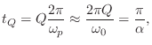
Another well known rule of thumb is that the ![]() of a resonator is the
number of ``periods'' under the exponential decay of its impulse
response. More precisely, we will show that, for
of a resonator is the
number of ``periods'' under the exponential decay of its impulse
response. More precisely, we will show that, for ![]() , the
impulse response decays by the factor
, the
impulse response decays by the factor ![]() in
in ![]() cycles, which
is about 96 percent decay, or -27 dB.
cycles, which
is about 96 percent decay, or -27 dB.
The impulse response corresponding to Eq.![]() (E.8) is found by
inverting the Laplace transform of the transfer function
(E.8) is found by
inverting the Laplace transform of the transfer function ![]() . Since it
is only second order, the solution can be found in many tables of
Laplace transforms. Alternatively, we can break it up into a sum of
first-order terms which are invertible by inspection (possibly after
rederiving the Laplace transform of an exponential decay, which is
very simple). Thus we perform the partial fraction expansion of
Eq.
. Since it
is only second order, the solution can be found in many tables of
Laplace transforms. Alternatively, we can break it up into a sum of
first-order terms which are invertible by inspection (possibly after
rederiving the Laplace transform of an exponential decay, which is
very simple). Thus we perform the partial fraction expansion of
Eq.![]() (E.8) to obtain
(E.8) to obtain
| (E.12) | |||
| (E.13) |
as the respective residues of the poles
The impulse response is thus
Assuming a resonator, ![]() , we have
, we have
![]() , where
, where
![]() (using notation of the
preceding section), and the impulse response reduces to
(using notation of the
preceding section), and the impulse response reduces to
We have shown so far that the impulse response ![]() decays as
decays as
![]() with a sinusoidal radian frequency
with a sinusoidal radian frequency
![]() under the exponential envelope. After Q periods at frequency
under the exponential envelope. After Q periods at frequency
![]() , time has advanced to
, time has advanced to
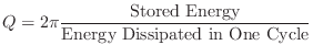
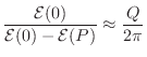
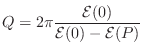
Q as Energy Stored over Energy Dissipated
Yet another meaning for ![]() is as follows [20, p. 326]
is as follows [20, p. 326]
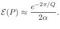
Proof. The total stored energy at time ![]() is
equal to the total energy of the remaining response. After an impulse
at time 0, the stored energy in a second-order resonator is
is
equal to the total energy of the remaining response. After an impulse
at time 0, the stored energy in a second-order resonator is
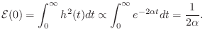
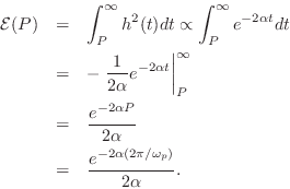
Assuming ![]() as before,
as before,
![]() so that
so that
Next Section:
Analog Allpass Filters
Previous Section:
Relating Pole Radius to Bandwidth


