


Alias Operator
Aliasing occurs when a signal is undersampled. If the signal
sampling rate ![]() is too low, we get frequency-domain
aliasing.
is too low, we get frequency-domain
aliasing.
The topic of aliasing normally arises in the context of sampling a continuous-time signal. The sampling theorem (Appendix D) says that we will have no aliasing due to sampling as long as the sampling rate is higher than twice the highest frequency present in the signal being sampled.
In this chapter, we are considering only discrete-time signals, in order to keep the math as simple as possible. Aliasing in this context occurs when a discrete-time signal is downsampled to reduce its sampling rate. You can think of continuous-time sampling as the limiting case for which the starting sampling rate is infinity.
An example of aliasing is shown in Fig.7.11. In the figure, the high-frequency sinusoid is indistinguishable from the lower-frequency sinusoid due to aliasing. We say the higher frequency aliases to the lower frequency.
![\includegraphics[scale=0.5]{eps/aliasing}](http://www.dsprelated.com/josimages_new/mdft/img1275.png)
Undersampling in the frequency domain gives rise to time-domain aliasing. If time or frequency is not specified, the term ``aliasing'' normally means frequency-domain aliasing (due to undersampling in the time domain).
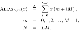
The aliasing operator for ![]() -sample signals
-sample signals
![]() is defined by
is defined by
Like the
![]() operator, the
operator, the
![]() operator maps a
length
operator maps a
length ![]() signal down to a length
signal down to a length ![]() signal. A way to think of
it is to partition the original
signal. A way to think of
it is to partition the original ![]() samples into
samples into ![]() blocks of length
blocks of length
![]() , with the first block extending from sample 0 to sample
, with the first block extending from sample 0 to sample ![]() ,
the second block from
,
the second block from ![]() to
to ![]() , etc. Then just add up the blocks.
This process is called aliasing. If the original signal
, etc. Then just add up the blocks.
This process is called aliasing. If the original signal ![]() is
a time signal, it is called time-domain aliasing; if it is a
spectrum, we call it frequency-domain aliasing, or just
aliasing. Note that aliasing is not invertible in general.
Once the blocks are added together, it is usually not possible to
recover the original blocks.
is
a time signal, it is called time-domain aliasing; if it is a
spectrum, we call it frequency-domain aliasing, or just
aliasing. Note that aliasing is not invertible in general.
Once the blocks are added together, it is usually not possible to
recover the original blocks.
Example:
![\begin{eqnarray*}
\hbox{\sc Alias}_2([0,1,2,3,4,5]) &=& [0,1,2] + [3,4,5] = [3,5...
...ox{\sc Alias}_3([0,1,2,3,4,5]) &=& [0,1] + [2,3] + [4,5] = [6,9]
\end{eqnarray*}](http://www.dsprelated.com/josimages_new/mdft/img1280.png)
The alias operator is used to state the Fourier theorem (§7.4.11)
![\includegraphics[width=4.5in]{eps/aliasingfd}](http://www.dsprelated.com/josimages_new/mdft/img1282.png) |
Figure 7.12 shows the result of
![]() applied to
applied to
![]() from Figure 7.9c. Imagine the spectrum of
Fig.7.12a as being plotted on a piece of paper rolled
to form a cylinder, with the edges of the paper meeting at
from Figure 7.9c. Imagine the spectrum of
Fig.7.12a as being plotted on a piece of paper rolled
to form a cylinder, with the edges of the paper meeting at ![]() (upper
right corner of Fig.7.12a). Then the
(upper
right corner of Fig.7.12a). Then the
![]() operation can be
simulated by rerolling the cylinder of paper to cut its circumference in
half. That is, reroll it so that at every point, two sheets of paper
are in contact at all points on the new, narrower cylinder. Now, simply
add the values on the two overlapping sheets together, and you have the
operation can be
simulated by rerolling the cylinder of paper to cut its circumference in
half. That is, reroll it so that at every point, two sheets of paper
are in contact at all points on the new, narrower cylinder. Now, simply
add the values on the two overlapping sheets together, and you have the
![]() of the original spectrum on the unit circle. To alias by
of the original spectrum on the unit circle. To alias by ![]() ,
we would shrink the cylinder further until the paper edges again line up,
giving three layers of paper in the cylinder, and so on.
,
we would shrink the cylinder further until the paper edges again line up,
giving three layers of paper in the cylinder, and so on.
Figure 7.12b shows what is plotted on the first circular wrap of the
cylinder of paper, and Fig.7.12c shows what is on the second wrap.
These are overlaid in Fig.7.12d and added together in
Fig.7.12e. Finally, Figure 7.12f shows both the addition
and the overlay of the two components. We say that the second component
(Fig.7.12c) ``aliases'' to new frequency components, while the
first component (Fig.7.12b) is considered to be at its original
frequencies. If the unit circle of Fig.7.12a covers frequencies
0 to ![]() , all other unit circles (Fig.7.12b-c) cover
frequencies 0 to
, all other unit circles (Fig.7.12b-c) cover
frequencies 0 to ![]() .
.
In general, aliasing by the factor ![]() corresponds to a
sampling-rate reduction by the factor
corresponds to a
sampling-rate reduction by the factor ![]() . To prevent aliasing
when reducing the sampling rate, an anti-aliasing lowpass
filter is generally used. The lowpass filter attenuates all signal
components at frequencies outside the interval
. To prevent aliasing
when reducing the sampling rate, an anti-aliasing lowpass
filter is generally used. The lowpass filter attenuates all signal
components at frequencies outside the interval
![]() so that all frequency components which would alias are first removed.
so that all frequency components which would alias are first removed.
Conceptually, in the frequency domain, the unit circle is reduced by
![]() to a unit circle
half the original size, where the two halves are summed. The inverse
of aliasing is then ``repeating'' which should be understood as
increasing the unit circle circumference using ``periodic
extension'' to generate ``more spectrum'' for the larger unit circle.
In the time domain, on the other hand, downsampling is the inverse of
the stretch operator. We may interchange ``time'' and ``frequency''
and repeat these remarks. All of these relationships are precise only
for integer stretch/downsampling/aliasing/repeat factors; in
continuous time and frequency, the restriction to integer factors is
removed, and we obtain the (simpler) scaling theorem (proved
in §C.2).
to a unit circle
half the original size, where the two halves are summed. The inverse
of aliasing is then ``repeating'' which should be understood as
increasing the unit circle circumference using ``periodic
extension'' to generate ``more spectrum'' for the larger unit circle.
In the time domain, on the other hand, downsampling is the inverse of
the stretch operator. We may interchange ``time'' and ``frequency''
and repeat these remarks. All of these relationships are precise only
for integer stretch/downsampling/aliasing/repeat factors; in
continuous time and frequency, the restriction to integer factors is
removed, and we obtain the (simpler) scaling theorem (proved
in §C.2).
Next Section:
Linearity
Previous Section:
Downsampling Operator


