


Correlation Analysis
The correlation operator (defined in §7.2.5) plays a major role in statistical signal processing. For a proper development, see, e.g., [27,33,65]. This section introduces only some of the most basic elements of statistical signal processing in a simplified manner, with emphasis on illustrating applications of the DFT.
Cross-Correlation
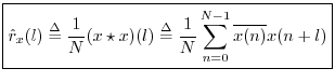
Definition: The circular cross-correlation of two signals ![]() and
and
![]() in
in ![]() may be defined by
may be defined by
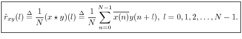
The term ``cross-correlation'' comes from
statistics, and what we have defined here is more properly
called a ``sample cross-correlation.''
That is,
![]() is an
estimator8.8 of the true
cross-correlation
is an
estimator8.8 of the true
cross-correlation ![]() which is an assumed statistical property
of the signal itself. This definition of a sample cross-correlation is only valid for
stationary stochastic processes, e.g., ``steady noises'' that
sound unchanged over time. The statistics of a stationary stochastic
process are by definition time invariant, thereby allowing
time-averages to be used for estimating statistics such
as cross-correlations. For brevity below, we will typically
not include ``sample'' qualifier, because all computational
methods discussed will be sample-based methods intended for use on
stationary data segments.
which is an assumed statistical property
of the signal itself. This definition of a sample cross-correlation is only valid for
stationary stochastic processes, e.g., ``steady noises'' that
sound unchanged over time. The statistics of a stationary stochastic
process are by definition time invariant, thereby allowing
time-averages to be used for estimating statistics such
as cross-correlations. For brevity below, we will typically
not include ``sample'' qualifier, because all computational
methods discussed will be sample-based methods intended for use on
stationary data segments.
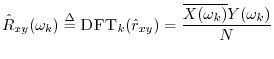
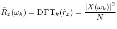
The DFT of the cross-correlation may be called the cross-spectral density, or ``cross-power spectrum,'' or even simply ``cross-spectrum'':
Unbiased Cross-Correlation
Recall that the cross-correlation operator is cyclic (circular)
since ![]() is interpreted modulo
is interpreted modulo ![]() . In practice, we are normally
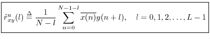
interested in estimating the acyclic cross-correlation
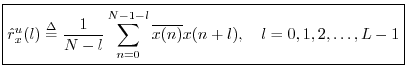
between two signals. For this (more realistic) case, we may define
instead the unbiased cross-correlation
. In practice, we are normally
interested in estimating the acyclic cross-correlation
between two signals. For this (more realistic) case, we may define
instead the unbiased cross-correlation
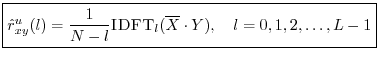
An unbiased acyclic cross-correlation may be computed faster via DFT (FFT) methods using zero padding:
![\begin{eqnarray*}
X &=& \hbox{\sc DFT}[\hbox{\sc CausalZeroPad}_{N+L-1}(x)]\\
Y &=& \hbox{\sc DFT}[\hbox{\sc CausalZeroPad}_{N+L-1}(y)].
\end{eqnarray*}](http://www.dsprelated.com/josimages_new/mdft/img1562.png)
Note that ![]() and
and ![]() belong to
belong to ![]() while
while ![]() and
and ![]() belong to
belong to
![]() . The zero-padding may be causal (as defined in
§7.2.8)
because the signals are assumed to be be stationary, in which case all
signal statistics are time-invariant. As usual when embedding acyclic
correlation (or convolution) within the cyclic variant given by the
DFT, sufficient zero-padding is provided so that only zeros are ``time
aliased'' (wrapped around in time) by modulo indexing.
. The zero-padding may be causal (as defined in
§7.2.8)
because the signals are assumed to be be stationary, in which case all
signal statistics are time-invariant. As usual when embedding acyclic
correlation (or convolution) within the cyclic variant given by the
DFT, sufficient zero-padding is provided so that only zeros are ``time
aliased'' (wrapped around in time) by modulo indexing.
Cross-correlation is used extensively in audio signal processing for applications such as time scale modification, pitch shifting, click removal, and many others.
Autocorrelation
The cross-correlation of a signal with itself gives its autocorrelation:
The unbiased cross-correlation similarly reduces to an unbiased
autocorrelation when ![]() :
:
The DFT of the true autocorrelation function
![]() is the (sampled)
power spectral density (PSD), or power spectrum, and may
be denoted
is the (sampled)
power spectral density (PSD), or power spectrum, and may
be denoted
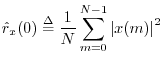
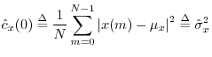
At lag zero, the autocorrelation function reduces to the average power (mean square) which we defined in §5.8:
Replacing ``correlation'' with ``covariance'' in the above definitions gives corresponding zero-mean versions. For example, we may define the sample circular cross-covariance as
![$\displaystyle \zbox {{\hat c}_{xy}(n)
\isdef \frac{1}{N}\sum_{m=0}^{N-1}\overline{[x(m)-\mu_x]} [y(m+n)-\mu_y].}
$](http://www.dsprelated.com/josimages_new/mdft/img1575.png)
Matched Filtering
The cross-correlation function is used extensively in pattern
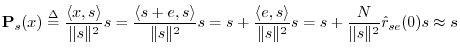
recognition and signal detection. We know from Chapter 5
that projecting one signal onto another is a means of measuring how
much of the second signal is present in the first. This can be used
to ``detect'' the presence of known signals as components of more
complicated signals. As a simple example, suppose we record ![]() which we think consists of a signal
which we think consists of a signal ![]() that we are looking for
plus some additive measurement noise
that we are looking for
plus some additive measurement noise ![]() . That is, we assume the
signal model
. That is, we assume the
signal model
![]() . Then the projection of
. Then the projection of ![]() onto
onto ![]() is
(recalling §5.9.9)
is
(recalling §5.9.9)
In the same way that FFT convolution is faster than direct convolution (see Table 7.1), cross-correlation and matched filtering are generally carried out most efficiently using an FFT algorithm (Appendix A).
FIR System Identification
Estimating an impulse response from input-output measurements is called system identification, and a large literature exists on this topic (e.g., [39]).
Cross-correlation can be used to compute the impulse response ![]() of a filter from the cross-correlation of its input and output signals
of a filter from the cross-correlation of its input and output signals
![]() and
and
![]() , respectively. To see this, note that, by
the correlation theorem,
, respectively. To see this, note that, by
the correlation theorem,

% sidex.m - Demonstration of the use of FFT cross- % correlation to compute the impulse response % of a filter given its input and output. % This is called "FIR system identification". Nx = 32; % input signal length Nh = 10; % filter length Ny = Nx+Nh-1; % max output signal length % FFT size to accommodate cross-correlation: Nfft = 2^nextpow2(Ny); % FFT wants power of 2 x = rand(1,Nx); % input signal = noise %x = 1:Nx; % input signal = ramp h = [1:Nh]; % the filter xzp = [x,zeros(1,Nfft-Nx)]; % zero-padded input yzp = filter(h,1,xzp); % apply the filter X = fft(xzp); % input spectrum Y = fft(yzp); % output spectrum Rxx = conj(X) .* X; % energy spectrum of x Rxy = conj(X) .* Y; % cross-energy spectrum Hxy = Rxy ./ Rxx; % should be the freq. response hxy = ifft(Hxy); % should be the imp. response hxy(1:Nh) % print estimated impulse response freqz(hxy,1,Nfft); % plot estimated freq response err = norm(hxy - [h,zeros(1,Nfft-Nh)])/norm(h); disp(sprintf(['Impulse Response Error = ',... '%0.14f%%'],100*err)); err = norm(Hxy-fft([h,zeros(1,Nfft-Nh)]))/norm(h); disp(sprintf(['Frequency Response Error = ',... '%0.14f%%'],100*err)); |
Next Section:
Power Spectral Density Estimation
Previous Section:
Filters and Convolution


