


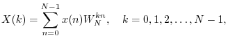
Fast Fourier Transform (FFT) Algorithms
The term fast Fourier transform (FFT) refers to an efficient
implementation of the discrete Fourier transform (DFT) for highly
compositeA.1 transform
lengths ![]() . When computing the DFT as a set of
. When computing the DFT as a set of ![]() inner products of
length
inner products of
length ![]() each, the computational complexity is
each, the computational complexity is
![]() . When
. When
![]() is an integer power of 2, a Cooley-Tukey FFT algorithm delivers
complexity
is an integer power of 2, a Cooley-Tukey FFT algorithm delivers
complexity
![]() , where
, where ![]() denotes the log-base-2 of
denotes the log-base-2 of
![]() , and
, and
![]() means ``on the order of
means ``on the order of ![]() ''.
Such FFT algorithms were evidently first used by Gauss in 1805
[30] and rediscovered in the 1960s by Cooley and Tukey
[16].
''.
Such FFT algorithms were evidently first used by Gauss in 1805
[30] and rediscovered in the 1960s by Cooley and Tukey
[16].
In this appendix, a brief introduction is given for various FFT algorithms. A tutorial review (1990) is given in [22]. Additionally, there are some excellent FFT ``home pages'':
Pointers to FFT software are given in §A.7.
Mixed-Radix Cooley-Tukey FFT
When the desired DFT length ![]() can be expressed as a product of
smaller integers, the Cooley-Tukey decomposition provides what is
called a mixed radix Cooley-Tukey FFT algorithm.A.2
can be expressed as a product of
smaller integers, the Cooley-Tukey decomposition provides what is
called a mixed radix Cooley-Tukey FFT algorithm.A.2
Two basic varieties of Cooley-Tukey FFT are decimation in time (DIT) and its Fourier dual, decimation in frequency (DIF). The next section illustrates decimation in time.
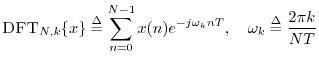
Decimation in Time
The DFT is defined by
When ![]() is even, the DFT summation can be split into sums over the
odd and even indexes of the input signal:
is even, the DFT summation can be split into sums over the
odd and even indexes of the input signal:
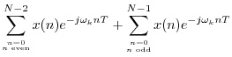
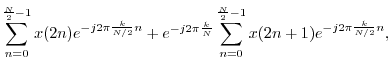
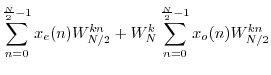
where
Radix 2 FFT
When ![]() is a power of
is a power of ![]() , say
, say ![]() where
where ![]() is an integer,
then the above DIT decomposition can be performed
is an integer,
then the above DIT decomposition can be performed ![]() times, until
each DFT is length
times, until
each DFT is length ![]() . A length
. A length ![]() DFT requires no multiplies. The
overall result is called a radix 2 FFT. A different radix 2
FFT is derived by performing decimation in frequency.
DFT requires no multiplies. The
overall result is called a radix 2 FFT. A different radix 2
FFT is derived by performing decimation in frequency.
A split radix FFT is theoretically more efficient than a pure radix 2 algorithm [73,31] because it minimizes real arithmetic operations. The term ``split radix'' refers to a DIT decomposition that combines portions of one radix 2 and two radix 4 FFTs [22].A.3On modern general-purpose processors, however, computation time is often not minimized by minimizing the arithmetic operation count (see §A.7 below).
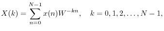
Radix 2 FFT Complexity is N Log N
Putting together the length ![]() DFT from the
DFT from the ![]() length-
length-![]() DFTs in
a radix-2 FFT, the only multiplies needed are those used to combine
two small DFTs to make a DFT twice as long, as in Eq.
DFTs in
a radix-2 FFT, the only multiplies needed are those used to combine
two small DFTs to make a DFT twice as long, as in Eq.![]() (A.1).
Since there are approximately
(A.1).
Since there are approximately ![]() (complex) multiplies needed for each
stage of the DIT decomposition, and only
(complex) multiplies needed for each
stage of the DIT decomposition, and only ![]() stages of DIT (where
stages of DIT (where
![]() denotes the log-base-2 of
denotes the log-base-2 of ![]() ), we see that the total number
of multiplies for a length
), we see that the total number
of multiplies for a length ![]() DFT is reduced from
DFT is reduced from
![]() to
to
![]() , where
, where
![]() means ``on the order of
means ``on the order of ![]() ''. More
precisely, a complexity of
''. More
precisely, a complexity of
![]() means that given any
implementation of a length-
means that given any
implementation of a length-![]() radix-2 FFT, there exist a constant
radix-2 FFT, there exist a constant ![]() and integer
and integer ![]() such that the computational complexity
such that the computational complexity
![]() satisfies
satisfies
Fixed-Point FFTs and NFFTs
Recall (e.g., from Eq.![]() (6.1)) that the inverse DFT requires a
division by
(6.1)) that the inverse DFT requires a
division by ![]() that the forward DFT does not. In fixed-point
arithmetic (Appendix G), and when
that the forward DFT does not. In fixed-point
arithmetic (Appendix G), and when ![]() is a power of 2,
dividing by
is a power of 2,
dividing by ![]() may be carried out by right-shifting
may be carried out by right-shifting ![]() places in the binary word. Fixed-point implementations of the inverse
Fast Fourier Transforms (FFT) (Appendix A) typically right-shift one
place after each Butterfly stage. However, superior overall numerical
performance may be obtained by right-shifting after every other
butterfly stage [8], which corresponds to dividing both the
forward and inverse FFT by
places in the binary word. Fixed-point implementations of the inverse
Fast Fourier Transforms (FFT) (Appendix A) typically right-shift one
place after each Butterfly stage. However, superior overall numerical
performance may be obtained by right-shifting after every other
butterfly stage [8], which corresponds to dividing both the
forward and inverse FFT by ![]() (i.e.,
(i.e., ![]() is implemented
by half as many right shifts as dividing by
is implemented
by half as many right shifts as dividing by ![]() ). Thus, in
fixed-point, numerical performance can be improved, no extra work is
required, and the normalization work (right-shifting) is spread
equally between the forward and reverse transform, instead of
concentrating all
). Thus, in
fixed-point, numerical performance can be improved, no extra work is
required, and the normalization work (right-shifting) is spread
equally between the forward and reverse transform, instead of
concentrating all ![]() right-shifts in the inverse transform. The NDFT
is therefore quite attractive for fixed-point implementations.
right-shifts in the inverse transform. The NDFT
is therefore quite attractive for fixed-point implementations.
Because signal amplitude can grow by a factor of 2 from one butterfly
stage to the next, an extra guard bit is needed for each pair of
subsequent NDFT butterfly stages. Also note that if the DFT length
![]() is not a power of
is not a power of ![]() , the number of right-shifts in the
forward and reverse transform must differ by one (because
, the number of right-shifts in the
forward and reverse transform must differ by one (because
![]() is odd instead of even).
is odd instead of even).
Prime Factor Algorithm (PFA)
By the prime factorization theorem, every integer ![]() can be uniquely
factored into a product of prime numbers
can be uniquely
factored into a product of prime numbers ![]() raised to an
integer power
raised to an
integer power ![]() :
:

It is interesting to note that the PFA actually predates the Cooley-Tukey FFT paper of 1965 [16], with Good's 1958 work on the PFA being cited in that paper [83].
The PFA and Winograd transform [43] are closely related, with the PFA being somewhat faster [9].
Rader's FFT Algorithm for Prime Lengths
Rader's FFT algorithm can be used to compute DFTs of length ![]() in
in
![]() operations when
operations when ![]() is a prime number.
For an introduction, see the Wikipedia page for Rader's FFT Algorithm:
is a prime number.
For an introduction, see the Wikipedia page for Rader's FFT Algorithm:
http://en.wikipedia.org/wiki/Rader's_FFT_algorithm
Bluestein's FFT Algorithm
Like Rader's FFT, Bluestein's FFT algorithm (also known as the
chirp ![]() -transform algorithm), can be used to compute
prime-length DFTs in
-transform algorithm), can be used to compute
prime-length DFTs in
![]() operations
[24, pp. 213-215].A.6 However,
unlike Rader's FFT, Bluestein's algorithm is not restricted to prime
lengths, and it can compute other kinds of transforms, as discussed
further below.
operations
[24, pp. 213-215].A.6 However,
unlike Rader's FFT, Bluestein's algorithm is not restricted to prime
lengths, and it can compute other kinds of transforms, as discussed
further below.
Beginning with the DFT
where `![]() ' denotes convolution (§7.2.4), and
the sequences
' denotes convolution (§7.2.4), and
the sequences ![]() and
and ![]() are defined by
are defined by

where the ranges of ![]() given are those actually required by the
convolution sum above. Beyond these required minimum ranges for
given are those actually required by the
convolution sum above. Beyond these required minimum ranges for ![]() ,
the sequences may be extended by zeros. As a result, we may implement
this convolution (which is cyclic for even
,
the sequences may be extended by zeros. As a result, we may implement
this convolution (which is cyclic for even ![]() and ``negacyclic'' for
odd
and ``negacyclic'' for
odd ![]() ) using zero-padding and a larger cyclic convolution, as
mentioned in §7.2.4. In particular, the larger cyclic
convolution size
) using zero-padding and a larger cyclic convolution, as
mentioned in §7.2.4. In particular, the larger cyclic
convolution size
![]() may be chosen a power of 2, which need
not be larger than
may be chosen a power of 2, which need
not be larger than ![]() . Within this larger cyclic convolution, the
negative-
. Within this larger cyclic convolution, the
negative-![]() indexes map to
indexes map to
![]() in the usual way.
in the usual way.
Note that the sequence ![]() above consists of the original data
sequence
above consists of the original data
sequence ![]() multiplied by a signal
multiplied by a signal
![]() which can be
interpreted as a sampled complex sinusoid with instantaneous
normalized radian frequency
which can be
interpreted as a sampled complex sinusoid with instantaneous
normalized radian frequency ![]() , i.e., an instantaneous
frequency that increases linearly with time. Such signals are called
chirp signals. For this reason, Bluestein's algorithm is also
called the chirp
, i.e., an instantaneous
frequency that increases linearly with time. Such signals are called
chirp signals. For this reason, Bluestein's algorithm is also
called the chirp ![]() -transform algorithm [59].
-transform algorithm [59].
In summary, Bluestein's FFT algorithm provides complexity ![]() for any positive integer DFT-length
for any positive integer DFT-length ![]() whatsoever, even when
whatsoever, even when ![]() is
prime.
is
prime.
Other adaptations of the Bluestein FFT algorithm can be used to
compute a contiguous subset of DFT frequency samples (any uniformly
spaced set of samples along the unit circle), with ![]() complexity. It can similarly compute samples of the
complexity. It can similarly compute samples of the ![]() transform
along a sampled spiral of the form
transform
along a sampled spiral of the form ![]() , where
, where ![]() is any complex
number, and
is any complex
number, and
![]() , again with complexity
, again with complexity ![]() [24].
[24].
Fast Transforms in Audio DSP
Since most audio signal processing applications benefit from zero padding (see §8.1), in which case we can always choose the FFT length to be a power of 2, there is almost never a need in practice for more ``exotic'' FFT algorithms than the basic ``pruned'' power-of-2 algorithms. (Here ``pruned'' means elimination of all unnecessary operations, such as when the input signal is real [74,21].)
An exception is when processing exactly periodic signals where the period is known to be an exact integer number of samples in length.A.8 In such a case, the DFT of one period of the waveform can be interpreted as a Fourier series (§B.3) of the periodic waveform, and unlike virtually all other practical spectrum analysis scenarios, spectral interpolation is not needed (or wanted). In the exactly periodic case, the spectrum is truly zero between adjacent harmonic frequencies, and the DFT of one period provides spectral samples only at the harmonic frequencies.
Adaptive FFT software (see §A.7 below) will choose the fastest algorithm available for any desired DFT length. Due to modern processor architectures, execution time is not normally minimized by minimizing arithmetic complexity [23].
Related Transforms
There are alternatives to the Cooley-Tukey FFT which can serve the same or related purposes and which can have advantages in certain situations [10]. Examples include the fast discrete cosine transform (DCT) [5], discrete Hartley transform [21], and number theoretic transform [2].
The DCT, used extensively in image coding, is described in §A.6.1 below. The Hartley transform, optimized for processing real signals, does not appear to have any advantages over a ``pruned real-only FFT'' [74]. The number theoretic transform has special applicability for large-scale, high-precision calculations (§A.6.2 below).
The Discrete Cosine Transform (DCT)
In image coding (such as MPEG and JPEG), and many audio coding
algorithms (MPEG), the discrete cosine transform (DCT) is used
because of its nearly optimal asymptotic theoretical
coding gain.A.9For 1D signals, one of several DCT definitions (the one called
DCT-II)A.10is given by
![$\displaystyle 2\sum_{n=0}^{N-1} x(n) \cos\left[\frac{\pi k}{2N}(2n+1)\right],
\quad k=0,1,2,\ldots,N-1$](http://www.dsprelated.com/josimages_new/mdft/img1668.png)
![$\displaystyle 2\sum_{n=0}^{N-1} x(n) \cos\left[\omega_k\left(n+\frac{1}{2}\right)\right]
\protect$](http://www.dsprelated.com/josimages_new/mdft/img1669.png)
where
For real signals, the real part of the DFT is a kind of DCT:
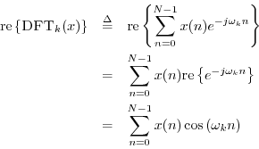
Thus, the real part of a double-length FFT is the same as the DCT
except for the half-sample phase shift in the sinusoidal basis
functions
![]() (and a scaling by 2 which is
unimportant).
(and a scaling by 2 which is
unimportant).
In practice, the DCT is normally implemented using the same basic efficiency techniques as in FFT algorithms. In Matlab and Octave (Octave-Forge), the functions dct and dct2 are available for the 1D and 2D cases, respectively.
Exercise: Using Euler's identity, expand the cosine
in the DCT defined by Eq.![]() (A.2) above into a sum of complex
sinusoids, and show that the DCT can be rewritten as the sum of two
phase-modulated DFTs:
(A.2) above into a sum of complex
sinusoids, and show that the DCT can be rewritten as the sum of two
phase-modulated DFTs:
Number Theoretic Transform
The number theoretic transform is based on generalizing the
![]() th primitive root of unity (see §3.12) to a
``quotient ring'' instead of the usual field of complex numbers. Let
th primitive root of unity (see §3.12) to a
``quotient ring'' instead of the usual field of complex numbers. Let
![]() denote a primitive
denote a primitive ![]() th root of unity. We have been using
th root of unity. We have been using
![]() in the field of complex numbers, and it of course
satisfies
in the field of complex numbers, and it of course
satisfies ![]() , making it a root of unity; it also has the
property that
, making it a root of unity; it also has the
property that ![]() visits all of the ``DFT frequency points'' on
the unit circle in the
visits all of the ``DFT frequency points'' on
the unit circle in the ![]() plane, as
plane, as ![]() goes from 0 to
goes from 0 to ![]() .
.
In a number theory transform, ![]() is an integer which
satisfies
is an integer which
satisfies
When the number of elements in the transform is composite, a ``fast number theoretic transform'' may be constructed in the same manner as a fast Fourier transform is constructed from the DFT, or as the prime factor algorithm (or Winograd transform) is constructed for products of small mutually prime factors [43].
Unlike the DFT, the number theoretic transform does not transform to a meaningful ``frequency domain''. However, it has analogous theorems, such as the convolution theorem, enabling it to be used for fast convolutions and correlations like the various FFT algorithms.
An interesting feature of the number theory transform is that all
computations are exact (integer multiplication and addition
modulo a prime integer). There is no round-off error. This feature
has been used to do fast convolutions to multiply extremely large
numbers, such as are needed when computing ![]() to millions of digits
of precision.
to millions of digits
of precision.
FFT Software
For those of us in signal processing research, the built-in fft function in Matlab (or Octave) is what we use almost all the time. It is adaptive in that it will choose the best algorithm available for the desired transform size.
For C or C++ applications, there are several highly optimized FFT variants in the FFTW package (``Fastest Fourier Transform in the West'') [23]. FFTW is free for non-commercial or free-software applications under the terms of the GNU General Public License.
For embedded DSP applications (software running on special purpose DSP chips), consult your vendor's software libraries and support website for FFT algorithms written in optimized assembly language for your DSP hardware platform. Nearly all DSP chip vendors supply free FFT software (and other signal processing utilities) as a way of promoting their hardware.
Next Section:
Fourier Transforms for Continuous/Discrete Time/Frequency
Previous Section:
Example Applications of the DFT


