


Importance of Generalized Complex Sinusoids
As a preview of things to come, note that one signal
![]() 4.15 is
projected onto another signal
4.15 is
projected onto another signal ![]() using an inner
product. The inner product
using an inner
product. The inner product
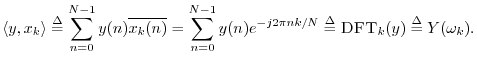
![]() computes the coefficient
of projection4.16 of
computes the coefficient
of projection4.16 of ![]() onto
onto ![]() . If
. If
![]() (a sampled, unit-amplitude, zero-phase, complex
sinusoid), then the inner product computes the Discrete Fourier
Transform (DFT), provided the frequencies are chosen to be
(a sampled, unit-amplitude, zero-phase, complex
sinusoid), then the inner product computes the Discrete Fourier
Transform (DFT), provided the frequencies are chosen to be
![]() . For the DFT, the inner product is specifically
. For the DFT, the inner product is specifically
Another case of importance is the Discrete Time Fourier Transform
(DTFT), which is like the DFT except that the transform accepts an
infinite number of samples instead of only ![]() . In this case,
frequency is continuous, and
. In this case,
frequency is continuous, and
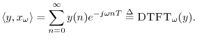
If, more generally,
![]() (a sampled complex sinusoid with
exponential growth or decay), then the inner product becomes
(a sampled complex sinusoid with
exponential growth or decay), then the inner product becomes
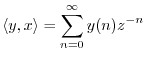
Why have a ![]() transform when it seems to contain no more information than
the DTFT? It is useful to generalize from the unit circle (where the DFT
and DTFT live) to the entire complex plane (the
transform when it seems to contain no more information than
the DTFT? It is useful to generalize from the unit circle (where the DFT
and DTFT live) to the entire complex plane (the ![]() transform's domain) for
a number of reasons. First, it allows transformation of growing
functions of time such as growing exponentials; the only limitation on
growth is that it cannot be faster than exponential. Secondly, the
transform's domain) for
a number of reasons. First, it allows transformation of growing
functions of time such as growing exponentials; the only limitation on
growth is that it cannot be faster than exponential. Secondly, the ![]() transform has a deeper algebraic structure over the complex plane as a
whole than it does only over the unit circle. For example, the
transform has a deeper algebraic structure over the complex plane as a
whole than it does only over the unit circle. For example, the ![]() transform of any finite signal is simply a polynomial in
transform of any finite signal is simply a polynomial in ![]() . As
such, it can be fully characterized (up to a constant scale factor) by its
zeros in the
. As
such, it can be fully characterized (up to a constant scale factor) by its
zeros in the ![]() plane. Similarly, the
plane. Similarly, the ![]() transform of an
exponential can be characterized to within a scale factor
by a single point in the
transform of an
exponential can be characterized to within a scale factor
by a single point in the ![]() plane (the
point which generates the exponential); since the
plane (the
point which generates the exponential); since the ![]() transform goes
to infinity at that point, it is called a pole of the transform.
More generally, the
transform goes
to infinity at that point, it is called a pole of the transform.
More generally, the ![]() transform of any generalized complex sinusoid
is simply a pole located at the point which generates the sinusoid.
Poles and zeros are used extensively in the analysis of recursive
digital filters. On the most general level, every finite-order, linear,
time-invariant, discrete-time system is fully specified (up to a scale
factor) by its poles and zeros in the
transform of any generalized complex sinusoid
is simply a pole located at the point which generates the sinusoid.
Poles and zeros are used extensively in the analysis of recursive
digital filters. On the most general level, every finite-order, linear,
time-invariant, discrete-time system is fully specified (up to a scale
factor) by its poles and zeros in the ![]() plane. This topic will be taken
up in detail in Book II [68].
plane. This topic will be taken
up in detail in Book II [68].
In the continuous-time case, we have the Fourier transform
which projects ![]() onto the continuous-time sinusoids defined by
onto the continuous-time sinusoids defined by
![]() , and the appropriate inner product is
, and the appropriate inner product is
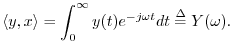
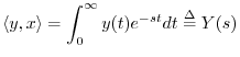
Finally, the Laplace transform is the continuous-time counterpart
of the ![]() transform, and it projects signals onto exponentially growing
or decaying complex sinusoids:
transform, and it projects signals onto exponentially growing
or decaying complex sinusoids:
Next Section:
Comparing Analog and Digital Complex Planes
Previous Section:
Phasor and Carrier Components of Sinusoids


