


Taylor Series Expansions
A Taylor series expansion of a continuous function ![]() is a
polynomial approximation of
is a
polynomial approximation of ![]() . This appendix derives
the Taylor series approximation informally, then introduces the
remainder term and a formal statement of Taylor's theorem. Finally, a
basic result on the completeness of polynomial approximation is
stated.
. This appendix derives
the Taylor series approximation informally, then introduces the
remainder term and a formal statement of Taylor's theorem. Finally, a
basic result on the completeness of polynomial approximation is
stated.
Informal Derivation of Taylor Series
We have a function ![]() and we want to approximate it using an
and we want to approximate it using an
![]() th-order polynomial:
th-order polynomial:
Our problem is to find fixed constants
![]() so as to obtain
the best approximation possible. Let's proceed optimistically as though
the approximation will be perfect, and assume
so as to obtain
the best approximation possible. Let's proceed optimistically as though
the approximation will be perfect, and assume
![]() for all
for all ![]() (
(
![]() ), given the right values of
), given the right values of ![]() . Then at
. Then at ![]() we
must have
we
must have
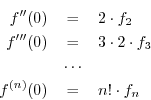
where
![]() denotes the
denotes the ![]() th derivative of
th derivative of ![]() with respect to
with respect to
![]() , evaluated at
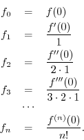
, evaluated at ![]() . Solving the above relations for the desired
constants yields
. Solving the above relations for the desired
constants yields
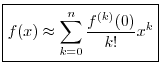
Thus, defining
![]() (as it always is), we have derived the
following polynomial approximation:
(as it always is), we have derived the
following polynomial approximation:
Taylor Series with Remainder
We repeat the derivation of the preceding section, but this time we treat the error term more carefully.
Again we want to approximate ![]() with an
with an ![]() th-order polynomial:
th-order polynomial:
Our problem is to find
![]() so as to minimize
so as to minimize
![]() over some interval
over some interval ![]() containing
containing ![]() . There are many
``optimality criteria'' we could choose. The one that falls out
naturally here is called Padé approximation. Padé
approximation sets the error value and its first
. There are many
``optimality criteria'' we could choose. The one that falls out
naturally here is called Padé approximation. Padé
approximation sets the error value and its first ![]() derivatives to
zero at a single chosen point, which we take to be
derivatives to
zero at a single chosen point, which we take to be ![]() . Since all
. Since all
![]() ``degrees of freedom'' in the polynomial coefficients
``degrees of freedom'' in the polynomial coefficients ![]() are
used to set derivatives to zero at one point, the approximation is
termed maximally flat at that point. In other words, as
are
used to set derivatives to zero at one point, the approximation is
termed maximally flat at that point. In other words, as
![]() , the
, the ![]() th order polynomial approximation approaches
th order polynomial approximation approaches ![]() with an error that is proportional to
with an error that is proportional to ![]() .
.
Padé approximation comes up elsewhere in signal processing. For example, it is the sense in which Butterworth filters are optimal [53]. (Their frequency responses are maximally flat in the center of the pass-band.) Also, Lagrange interpolation filters (which are nonrecursive, while Butterworth filters are recursive), can be shown to maximally flat at dc in the frequency domain [82,36].
Setting ![]() in the above polynomial approximation produces
in the above polynomial approximation produces
Differentiating the polynomial approximation and setting ![]() gives
gives
In the same way, we find
From this derivation, it is clear that the approximation error (remainder
term) is smallest in the vicinity of ![]() . All degrees of freedom
in the polynomial coefficients were devoted to minimizing the approximation
error and its derivatives at
. All degrees of freedom
in the polynomial coefficients were devoted to minimizing the approximation
error and its derivatives at ![]() . As you might expect, the approximation
error generally worsens as
. As you might expect, the approximation
error generally worsens as ![]() gets farther away from 0.
gets farther away from 0.
To obtain a more uniform approximation over some interval ![]() in
in ![]() , other kinds of error criteria may be employed. Classically,
this topic has been called ``economization of series,'' or simply
polynomial approximation under different error criteria. In
Matlab or
Octave, the function
polyfit(x,y,n) will find the coefficients of a polynomial
, other kinds of error criteria may be employed. Classically,
this topic has been called ``economization of series,'' or simply
polynomial approximation under different error criteria. In
Matlab or
Octave, the function
polyfit(x,y,n) will find the coefficients of a polynomial ![]() of
degree n that fits the data y over the points x in a
least-squares sense. That is, it minimizes
of
degree n that fits the data y over the points x in a
least-squares sense. That is, it minimizes

Formal Statement of Taylor's Theorem
Let ![]() be continuous on a real interval
be continuous on a real interval ![]() containing
containing ![]() (and
(and ![]() ),
and let
),
and let
![]() exist at
exist at ![]() and
and
![]() be continuous for
all
be continuous for
all ![]() . Then we have the following Taylor series expansion:
. Then we have the following Taylor series expansion:
![\begin{eqnarray*}
f(x) = f(x_0) &+& \frac{1}{1}f^\prime(x_0)(x-x_0) \\ [10pt]
&...
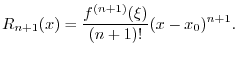
...&+& \frac{1}{n!}f^{(n+1)}(x_0)(x-x_0)^n\\ [10pt]
&+& R_{n+1}(x)
\end{eqnarray*}](http://www.dsprelated.com/josimages_new/mdft/img1874.png)
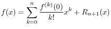
where
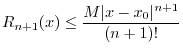
![]() is called the remainder term. Then Taylor's
theorem [63, pp. 95-96] provides that there exists some
is called the remainder term. Then Taylor's
theorem [63, pp. 95-96] provides that there exists some ![]() between
between ![]() and
and ![]() such that
such that
When ![]() , the Taylor series reduces to what is called a Maclaurin
series [56, p. 96].
, the Taylor series reduces to what is called a Maclaurin
series [56, p. 96].
Weierstrass Approximation Theorem
The Weierstrass approximation theorem assures us that polynomial approximation can get arbitrarily close to any continuous function as the polynomial order is increased.
Let ![]() be continuous on a real interval
be continuous on a real interval ![]() . Then for any
. Then for any
![]() , there exists an
, there exists an ![]() th-order polynomial
th-order polynomial ![]() , where
, where
![]() depends on
depends on ![]() , such that
, such that
For a proof, see, e.g., [63, pp. 146-148].
Thus, any continuous function can be approximated arbitrarily well by
means of a polynomial. This does not necessarily mean that a Taylor
series expansion can be used to find such a polynomial since, in
particular, the function must be differentiable of all orders
throughout ![]() . Furthermore, there can be points, even in infinitely
differentiable functions, about which a Taylor expansion will not
yield a good approximation, as illustrated in the next section. The
main point here is that, thanks to the Weierstrass approximation
theorem, we know that good polynomial approximations exist for
any continuous function.
. Furthermore, there can be points, even in infinitely
differentiable functions, about which a Taylor expansion will not
yield a good approximation, as illustrated in the next section. The
main point here is that, thanks to the Weierstrass approximation
theorem, we know that good polynomial approximations exist for
any continuous function.
Points of Infinite Flatness
Consider the inverted Gaussian pulse,E.1
As mentioned in §E.2, a measure of ``flatness'' is the number
of leading zero terms in a function's Taylor expansion (not counting
the first (constant) term). Thus, by this measure, the bell curve is
``infinitely flat'' at infinity, or, equivalently, ![]() is
infinitely flat at
is
infinitely flat at ![]() .
.
Another property of
![]() is that it has an
infinite number of ``zeros'' at
is that it has an
infinite number of ``zeros'' at ![]() . The fact that a function
. The fact that a function
![]() has an infinite number of zeros at
has an infinite number of zeros at ![]() can be verified by
showing
can be verified by
showing
The reciprocal of a function containing an infinite-order zero at
![]() has what is called an essential singularity at
has what is called an essential singularity at ![]() [15, p. 157], also called a
non-removable
singularity. Thus,
[15, p. 157], also called a
non-removable
singularity. Thus,
![]() has an essential
singularity at
has an essential
singularity at ![]() , and
, and ![]() has one at
has one at ![]() .
.
An amazing result from the theory of complex variables
[15, p. 270]
is that near an essential singular point
![]() (i.e.,
(i.e., ![]() may be
a complex number), the inequality
may be
a complex number), the inequality
In summary, a Taylor series expansion about the point ![]() will
always yield a constant approximation when the function being
approximated is infinitely flat at
will
always yield a constant approximation when the function being
approximated is infinitely flat at ![]() . For this reason, polynomial
approximations are often applied over a restricted range of
. For this reason, polynomial
approximations are often applied over a restricted range of ![]() , with
constraints added to provide transitions from one interval to the
next. This leads to the general subject of splines
[81]. In particular, cubic spline approximations
are composed of successive segments which are each third-order polynomials. In each segment,
four degrees of freedom are available (the four polynomial
coefficients). Two of these are usually devoted to matching the
amplitude and slope of the polynomial to one side, while the other two
are used to maximize some measure of fit across the segment. The
points at which adjacent polynomial segments connect are called
``knots'', and finding optimal knot locations is usually a relatively
expensive, iterative computation.
, with
constraints added to provide transitions from one interval to the
next. This leads to the general subject of splines
[81]. In particular, cubic spline approximations
are composed of successive segments which are each third-order polynomials. In each segment,
four degrees of freedom are available (the four polynomial
coefficients). Two of these are usually devoted to matching the
amplitude and slope of the polynomial to one side, while the other two
are used to maximize some measure of fit across the segment. The
points at which adjacent polynomial segments connect are called
``knots'', and finding optimal knot locations is usually a relatively
expensive, iterative computation.
Differentiability of Audio Signals
As mentioned in §3.6, every audio signal can be regarded as
infinitely differentiable due to the finite bandwidth of human
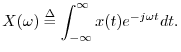
hearing. That is, given any audio signal ![]() , its Fourier
transform is given by
, its Fourier
transform is given by

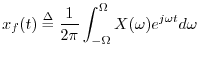
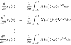
Since the length of the integral is finite, there is no possibility
that it can ``blow up'' due to the weighting by ![]() in the
frequency domain introduced by differentiation in the time domain.
in the
frequency domain introduced by differentiation in the time domain.
A basic Fourier property of signals and their spectra is that
a signal cannot be both time limited and frequency limited.
Therefore, by conceptually ``lowpass filtering'' every audio signal to
reject all frequencies above ![]() kHz, we implicitly make every audio
signal last forever! Another way of saying this is that the ``ideal
lowpass filter `rings' forever''. Such fine points do not concern us
in practice, but they are important for fully understanding the
underlying theory. Since, in reality, signals can be said to have a
true beginning and end, we must admit that all signals we really work
with in practice have infinite-bandwidth. That is, when a signal is
turned on or off, there is a spectral event extending all the way to
infinite frequency (while ``rolling off'' with frequency and having a
finite total energy).E.2
kHz, we implicitly make every audio
signal last forever! Another way of saying this is that the ``ideal
lowpass filter `rings' forever''. Such fine points do not concern us
in practice, but they are important for fully understanding the
underlying theory. Since, in reality, signals can be said to have a
true beginning and end, we must admit that all signals we really work
with in practice have infinite-bandwidth. That is, when a signal is
turned on or off, there is a spectral event extending all the way to
infinite frequency (while ``rolling off'' with frequency and having a
finite total energy).E.2
In summary, audio signals are perceptually equivalent to bandlimited
signals, and bandlimited signals are infinitely smooth in the sense
that derivatives of all orders exist at all points time
![]() .
.
Next Section:
Logarithms and Decibels
Previous Section:
Sampling Theory


