


First-Order Allpass Interpolation
A delay line interpolated by a first-order allpass filter is drawn in Fig.4.3.
![\includegraphics[width=\twidth]{eps/delayai}](http://www.dsprelated.com/josimages_new/pasp/img938.png)
Intuitively, ramping the coefficients of the allpass gradually ``grows'' or ``hides'' one sample of delay. This tells us how to handle resets when crossing sample boundaries.
The difference equation is
![\begin{eqnarray*}
{\hat x}(n-\Delta) \isdef y(n) &=& \eta \cdot x(n) + x(n-1) - ...
...y(n-1) \\
&=& \eta \cdot \left[ x(n) - y(n-1)\right] + x(n-1).
\end{eqnarray*}](http://www.dsprelated.com/josimages_new/pasp/img939.png)
Thus, like linear interpolation, first-order allpass interpolation requires only one multiply and two adds per sample of output.
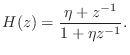
The transfer function is
At low frequencies (
Figure 4.4 shows the phase delay of the first-order digital allpass filter for a variety of desired delays at dc. Since the amplitude response of any allpass is 1 at all frequencies, there is no need to plot it.
![\includegraphics[width=\twidth]{eps/allpass1}](http://www.dsprelated.com/josimages_new/pasp/img943.png)
The first-order allpass interpolator is generally controlled by
setting its dc delay to the desired delay. Thus, for a given desired
delay ![]() , the allpass coefficient is (from
Eq.
, the allpass coefficient is (from
Eq.![]() (4.3))
(4.3))

Note that, unlike linear interpolation, allpass interpolation is not suitable for ``random access'' interpolation in which interpolated values may be requested at any arbitrary time in isolation. This is because the allpass is recursive so that it must run for enough samples to reach steady state. However, when the impulse response is reasonably short, as it is for delays near one sample, it can in fact be used in ``random access mode'' by giving it enough samples with which to work.
![\includegraphics[width=4.8in]{eps/ap1pz}](http://www.dsprelated.com/josimages_new/pasp/img949.png)
The STK class implementing allpass-interpolated delay is DelayA.
Minimizing First-Order Allpass Transient Response
In addition to approaching a pole-zero cancellation at ![]() , another
undesirable artifact appears as
, another
undesirable artifact appears as
![]() : The transient
response also becomes long when the pole at
: The transient
response also becomes long when the pole at ![]() gets close to
the unit circle.
gets close to
the unit circle.
A plot of the impulse response for
![]() is shown in
Fig.4.6. We see a lot of ``ringing'' near half the sampling rate.
We actually should expect this from the nonlinear-phase
distortion which is clearly evident near half the sampling rate in
Fig.4.4. We can interpret this phenomenon as the signal
components near half the sampling rate being delayed by different
amounts than other frequencies, therefore ``sliding out of alignment''
with them.
is shown in
Fig.4.6. We see a lot of ``ringing'' near half the sampling rate.
We actually should expect this from the nonlinear-phase
distortion which is clearly evident near half the sampling rate in
Fig.4.4. We can interpret this phenomenon as the signal
components near half the sampling rate being delayed by different
amounts than other frequencies, therefore ``sliding out of alignment''
with them.
![\includegraphics[width=\twidth]{eps/ap1ir}](http://www.dsprelated.com/josimages_new/pasp/img952.png)
For audio applications, we would like to keep the impulse-response
duration short enough to sound ``instantaneous.'' That is, we do not
wish to have audible ``ringing'' in the time domain near ![]() . For
high quality sampling rates, such as larger than
. For
high quality sampling rates, such as larger than ![]() kHz, there
is no issue of direct audibility, since the ringing is above the range
of human hearing. However, it is often convenient, especially for
research prototyping, to work at lower sampling rates where
kHz, there
is no issue of direct audibility, since the ringing is above the range
of human hearing. However, it is often convenient, especially for
research prototyping, to work at lower sampling rates where ![]() is
audible. Also, many commercial products use such sampling rates to
save costs.
is
audible. Also, many commercial products use such sampling rates to
save costs.
Since the time constant of decay, in samples, of the impulse response
of a pole of radius ![]() is approximately
is approximately
For example, suppose 100 ms is chosen as the maximum ![]() allowed
at a sampling rate of
allowed
at a sampling rate of
![]() . Then applying the above constraints
yields
. Then applying the above constraints
yields
![]() , corresponding to the allowed delay range
, corresponding to the allowed delay range
![]() .
.
Next Section:
Linear Interpolation as Resampling
Previous Section:
Linear Interpolation


