


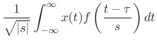
Continuous Wavelet Transform
In the present (Hilbert space) setting, we can now easily define the continuous wavelet transform in terms of its signal basis set:
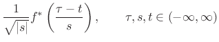 |
|||
 |
The parameter
![\includegraphics[width=0.8\twidth]{eps/wavelets}](http://www.dsprelated.com/josimages_new/sasp2/img2341.png)
The so-called admissibility condition for a mother wavelet
![]() is
is
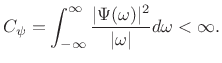
Given sufficient decay with
The Morlet wavelet is simply a Gaussian-windowed complex sinusoid:
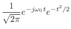 |
|||
The scale factor is chosen so that
| (12.119) |
In this case, we have
Since the scale parameter of a wavelet transform is analogous to frequency in a Fourier transform, a wavelet transform display is often called a scalogram, in analogy with an STFT ``spectrogram'' (discussed in §7.2).
When the mother wavelet can be interpreted as a windowed sinusoid (such as the Morlet wavelet), the wavelet transform can be interpreted as a constant-Q Fourier transform.12.5Before the theory of wavelets, constant-Q Fourier transforms (such as obtained from a classic third-octave filter bank) were not easy to invert, because the basis signals were not orthogonal. See Appendix E for related discussion.
Next Section:
Discrete Wavelet Transform
Previous Section:
Normalized STFT Basis


