


Dolph-Chebyshev Window
The Dolph-Chebyshev Window (or Chebyshev window, or
Dolph window) minimizes the Chebyshev norm of the side
lobes for a given main-lobe width ![]() [61,101],
[224, p. 94]:
[61,101],
[224, p. 94]:
 |
(4.43) |
The Chebyshev norm is also called the
An equivalent formulation is to minimize main-lobe width subject to a side-lobe specification:
 |
(4.44) |
The optimal Dolph-Chebyshev window transform can be written in closed form [61,101,105,156]:
![\begin{eqnarray*}
W(\omega_k) &=& \frac{\cos\left\{M\cos^{-1}\left[\beta\cos\left(\frac{\pi k}{M}\right)
\right]\right\}}{\cosh\left[M\cosh^{-1} (\beta)\right]},
\qquad k=0,1,2,\ldots,M-1 \\
\beta &=& \cosh \left[\frac{1}{M}\cosh^{-1}(10^\alpha)\right], \qquad (\alpha\approx 2,3,4).
\end{eqnarray*}](http://www.dsprelated.com/josimages_new/sasp2/img520.png)
The zero-phase Dolph-Chebyshev window, ![]() , is then computed as the
inverse DFT of
, is then computed as the
inverse DFT of
![]() .4.14 The
.4.14 The ![]() parameter controls the side-lobe level via the formula [156]
parameter controls the side-lobe level via the formula [156]
| Side-Lobe Level in dB |
(4.45) |
Thus,
The Chebyshev window can be regarded as the impulse response of an optimal Chebyshev lowpass filter having a zero-width pass-band (i.e., the main lobe consists of two ``transition bands''--see Chapter 4 regarding FIR filter design more generally).
Matlab for the Dolph-Chebyshev Window
In Matlab, the function chebwin(M,ripple) computes a length
![]() Dolph-Chebyshev window having a side-lobe level ripple dB below
that of the main-lobe peak. For example,
Dolph-Chebyshev window having a side-lobe level ripple dB below
that of the main-lobe peak. For example,
w = chebwin(31,60);designs a length
Example Chebyshev Windows and Transforms
Figure 3.31 shows the Dolph-Chebyshev window and its transform as designed by chebwin(31,40) in Matlab, and Fig.3.32 shows the same thing for chebwin(31,200). As can be seen from these examples, higher side-lobe levels are associated with a narrower main lobe and more discontinuous endpoints.
![\includegraphics[width=\twidth]{eps/cheb31R40}](http://www.dsprelated.com/josimages_new/sasp2/img528.png)
![\includegraphics[width=\twidth]{eps/cheb31R200}](http://www.dsprelated.com/josimages_new/sasp2/img529.png)
![\includegraphics[width=\twidth]{eps/cheb101R40}](http://www.dsprelated.com/josimages_new/sasp2/img530.png)
Figure 3.33 shows the Dolph-Chebyshev window and its transform as designed by chebwin(101,40) in Matlab. Note how the endpoints have actually become impulsive for the longer window length. The Hamming window, in contrast, is constrained to be monotonic away from its center in the time domain.
The ``equal ripple'' property in the frequency domain perfectly satisfies worst-case side-lobe specifications. However, it has the potentially unfortunate consequence of introducing ``impulses'' at the window endpoints. Such impulses can be the source of ``pre-echo'' or ``post-echo'' distortion which are time-domain effects not reflected in a simple side-lobe level specification. This is a good lesson in the importance of choosing the right error criterion to minimize. In this case, to avoid impulse endpoints, we might add a continuity or monotonicity constraint in the time domain (see §3.13.2 for examples).
Chebyshev and Hamming Windows Compared
Figure 3.34 shows an overlay of Hamming and Dolph-Chebyshev window transforms,
the ripple parameter for chebwin set to ![]() dB to make it
comparable to the Hamming side-lobe level. We see that the
monotonicity constraint inherent in the Hamming window family only
costs a few dB of deviation from optimality in the Chebyshev sense at
high frequency.
dB to make it
comparable to the Hamming side-lobe level. We see that the
monotonicity constraint inherent in the Hamming window family only
costs a few dB of deviation from optimality in the Chebyshev sense at
high frequency.
![\begin{psfrags}
% latex2html id marker 9837\psfrag{freq}{$\omega T$\ (radians per sample)}\begin{figure}[htbp]
\includegraphics[width=\twidth]{eps/chebHammingC}
\caption{}
\end{figure}
\end{psfrags}](http://www.dsprelated.com/josimages_new/sasp2/img532.png)
Dolph-Chebyshev Window Theory
In this section, the main elements of the theory behind the Dolph-Chebyshev window are summarized.
Chebyshev Polynomials
![\includegraphics[width=\twidth]{eps/first-even-chebs-c}](http://www.dsprelated.com/josimages_new/sasp2/img533.png)
The ![]() th Chebyshev polynomial may be defined by
th Chebyshev polynomial may be defined by
![$\displaystyle T_n(x) = \left\{\begin{array}{ll} \cos[n\cos^{-1}(x)], & \vert x\vert\le1 \\ [5pt] \cosh[n\cosh^{-1}(x)], & \vert x\vert>1 \\ \end{array} \right..$](http://www.dsprelated.com/josimages_new/sasp2/img534.png) |
(4.46) |
The first three even-order cases are plotted in Fig.3.35. (We will only need the even orders for making Chebyshev windows, as only they are symmetric about time 0.) Clearly,
| (4.47) |
for
 is an
is an  th-order polynomial in
  .
.
-
is an even function when
is an even integer,
and odd when
is odd.
-
has
zeros in the open interval
 , and
, and
 extrema in the closed interval
 ![$ [-1,1]$](http://www.dsprelated.com/josimages_new/sasp2/img543.png) .
.
 for
for  .
.
Dolph-Chebyshev Window Definition
Let ![]() denote the desired window length. Then the zero-phase
Dolph-Chebyshev window is defined in the frequency domain by
[155]
denote the desired window length. Then the zero-phase
Dolph-Chebyshev window is defined in the frequency domain by
[155]
![$\displaystyle W(\omega) = \frac{T_{M-1}[x_0 \cos(\omega/2)]}{T_{M-1}(x_0)}$](http://www.dsprelated.com/josimages_new/sasp2/img546.png) |
(4.48) |
where
 |
(4.49) |
where
![$\displaystyle \omega_c \isdefs 2\cos^{-1}\left[\frac{1}{x_0}\right].$](http://www.dsprelated.com/josimages_new/sasp2/img549.png) |
(4.50) |
Expanding
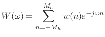 |
(4.51) |
where
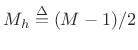 . Thus, the coefficients
Dolph-Chebyshev Window Main-Lobe Width
Given the window length ![]() and ripple magnitude
and ripple magnitude ![]() , the main-lobe
width
, the main-lobe
width ![]() may be computed as follows [155]:
may be computed as follows [155]:
![\begin{eqnarray*}
x_0 &=& \cosh\left[\frac{\cosh^{-1}\left(\frac{1}{r}\right)}{M-1}\right]\\
\omega_c &=& 2\cos^{-1}\left(\frac{1}{x_0}\right)
\end{eqnarray*}](http://www.dsprelated.com/josimages_new/sasp2/img553.png)
This is the smallest main-lobe width possible for the given window length and side-lobe spec.
Dolph-Chebyshev Window Length Computation
Given a prescribed side-lobe ripple-magnitude ![]() and main-lobe width
and main-lobe width
![]() , the required window length
, the required window length ![]() is given by [155]
is given by [155]
![$\displaystyle M = 1 + \frac{\cosh^{-1}(1/r)}{\cosh^{-1}[\sec(\omega_c/2)]}.$](http://www.dsprelated.com/josimages_new/sasp2/img554.png) |
(4.52) |
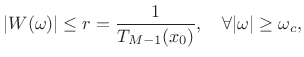
For
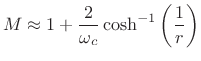 |
(4.53) |
Thus, half the time-bandwidth product in radians is approximately
 |
(4.54) |
where
Next Section:
Gaussian Window and Transform
Previous Section:
Kaiser Window


