


The Rectangular Window
The (zero-centered) rectangular window may be defined by
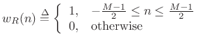 |
(4.2) |
where
![\includegraphics[width=3.5in]{eps/rectWindow}](http://www.dsprelated.com/josimages_new/sasp2/img306.png)
To see what happens in the frequency domain, we need to look at the DTFT of the window:
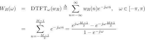
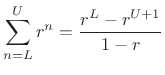
where the last line was derived using the closed form of a geometric series:
 |
(4.3) |
We can factor out linear phase terms from the numerator and denominator of the above expression to get
![$\displaystyle \frac{e^{-j \omega \frac{1}{2}}}{e^{-j\omega \frac{1}{2}}}
\left[ \frac{ e^{j \omega \frac{M}{2}}-e^{-j\omega\frac{M}{2}}}
{e^{j \omega\frac{1}{2}}-e^{-j\omega\frac{1}{2}}} \right]$](http://www.dsprelated.com/josimages_new/sasp2/img311.png)
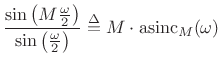
where
(also called the Dirichlet function [175,72] or periodic sinc function). This (real) result is for the zero-centered rectangular window. For the causal case, a linear phase term appears:
| (4.6) |
The term ``aliased sinc function'' refers to the fact that it may be
simply obtained by sampling the length-![]() continuous-time rectangular window, which has Fourier transform
sinc
continuous-time rectangular window, which has Fourier transform
sinc![]() (given amplitude
(given amplitude
![]() in the time domain). Sampling at intervals of
in the time domain). Sampling at intervals of ![]() seconds in
the time domain corresponds to aliasing in the frequency domain over
the interval
seconds in
the time domain corresponds to aliasing in the frequency domain over
the interval ![]() Hz, and by direct derivation, we have found the
result. It is interesting to consider what happens as the window
duration increases continuously in the time domain: the magnitude
spectrum can only change in discrete jumps as new samples are
included, even though it is continuously parametrized in
Hz, and by direct derivation, we have found the
result. It is interesting to consider what happens as the window
duration increases continuously in the time domain: the magnitude
spectrum can only change in discrete jumps as new samples are
included, even though it is continuously parametrized in ![]() .
.
As the sampling rate goes to infinity, the aliased sinc function therefore approaches the sinc function
Specifically,
 sinc
sincwhere
![\includegraphics[width=\textwidth ,height=2.25in]{eps/rectWindowRawFT}](http://www.dsprelated.com/josimages_new/sasp2/img329.png)
Figure 3.2 illustrates
![]() for
for ![]() . Note that this is the complete
window transform, not just its real part. We obtain real window
transforms like this only for zero-centered, symmetric windows. Note
that the phase of rectangular-window transform
. Note that this is the complete
window transform, not just its real part. We obtain real window
transforms like this only for zero-centered, symmetric windows. Note
that the phase of rectangular-window transform
![]() is
zero for
is
zero for
![]() , which is the width of the
main lobe. This is why zero-centered windows are often called
zero-phase windows; while the phase
actually alternates between 0
and
, which is the width of the
main lobe. This is why zero-centered windows are often called
zero-phase windows; while the phase
actually alternates between 0
and ![]() radians, the
radians, the ![]() values
occur only within side-lobes which are routinely neglected (in fact,
the window is normally designed to ensure that all side-lobes can be
neglected).
values
occur only within side-lobes which are routinely neglected (in fact,
the window is normally designed to ensure that all side-lobes can be
neglected).
More generally, we may plot both the magnitude and phase of the window versus frequency, as shown in Figures 3.4 and 3.5 below. In audio work, we more typically plot the window transform magnitude on a decibel (dB) scale, as shown in Fig.3.3 below. It is common to normalize the peak of the dB magnitude to 0 dB, as we have done here.
![\includegraphics[width=\twidth]{eps/rectWindowFT}](http://www.dsprelated.com/josimages_new/sasp2/img334.png)
![% latex2html id marker 73365
\includegraphics[width=\twidth,height=0.3125\theight]{eps/rectWindowFTzeroX}](http://www.dsprelated.com/josimages_new/sasp2/img335.png)
![% latex2html id marker 73369
\includegraphics[width=\twidth,height=0.3125\theight]{eps/rectWindowPhaseFT}](http://www.dsprelated.com/josimages_new/sasp2/img336.png)
Rectangular Window Side-Lobes
From Fig.3.3 and Eq.![]() (3.4), we see that the
main-lobe width is
(3.4), we see that the
main-lobe width is
![]() radian, and the
side-lobe level is 13 dB down.
radian, and the
side-lobe level is 13 dB down.
Since the DTFT of the rectangular window approximates the
sinc
function (see (3.4)), which has an amplitude envelope
proportional to ![]() (see (3.7)), it should ``roll
off'' at approximately 6 dB per octave (since
(see (3.7)), it should ``roll
off'' at approximately 6 dB per octave (since
![]() ). This is verified in the log-log
plot of Fig.3.6.
). This is verified in the log-log
plot of Fig.3.6.
![\includegraphics[width=\textwidth ]{eps/rectWindowLLFT}](http://www.dsprelated.com/josimages_new/sasp2/img341.png)
As the sampling rate approaches infinity, the rectangular window
transform (
![]() ) converges exactly to the
sinc
function.
Therefore, the departure of the roll-off from that of the
sinc
function can be ascribed to aliasing in the frequency domain,
due to sampling in the time domain (hence the name ``
) converges exactly to the
sinc
function.
Therefore, the departure of the roll-off from that of the
sinc
function can be ascribed to aliasing in the frequency domain,
due to sampling in the time domain (hence the name ``
![]() '').
'').
Note that each side lobe has width
![]() , as
measured between zero crossings.4.3 The main lobe, on the other hand, is
width
, as
measured between zero crossings.4.3 The main lobe, on the other hand, is
width ![]() . Thus, in principle, we should never confuse
side-lobe peaks with main-lobe peaks, because a peak must be at least
. Thus, in principle, we should never confuse
side-lobe peaks with main-lobe peaks, because a peak must be at least
![]() wide in order to be considered ``real''. However, in
complicated real-world scenarios, side-lobes can still cause
estimation errors (``bias''). Furthermore, two sinusoids at closely
spaced frequencies and opposite phase can partially cancel each
other's main lobes, making them appear to be narrower than
wide in order to be considered ``real''. However, in
complicated real-world scenarios, side-lobes can still cause
estimation errors (``bias''). Furthermore, two sinusoids at closely
spaced frequencies and opposite phase can partially cancel each
other's main lobes, making them appear to be narrower than
![]() .
.
In summary, the DTFT of the ![]() -sample rectangular window is
proportional to the `aliased sinc function':
-sample rectangular window is
proportional to the `aliased sinc function':
![\begin{eqnarray*}
\hbox{asinc}_M(\omega) &\isdef & \frac{\sin(\omega M / 2)}{M\cdot\sin(\omega/2)} \\ [0.2in]
&\approx& \frac{\sin(\pi fM)}{M\pi f} \isdefs \mbox{sinc}(fM)
\end{eqnarray*}](http://www.dsprelated.com/josimages_new/sasp2/img347.png)
Thus, it has zero crossings at integer multiples of
 |
(4.11) |
Its main-lobe width is
Rectangular Window Summary
The rectangular window was discussed in Chapter 5 (§3.1). Here we summarize the results of that discussion.
Definition (![]() odd):
odd):
![$\displaystyle w_R(n) \isdef \left\{\begin{array}{ll} 1, & \left\vert n\right\vert\leq\frac{M-1}{2} \\ [5pt] 0, & \hbox{otherwise} \\ \end{array} \right.$](http://www.dsprelated.com/josimages_new/sasp2/img349.png) |
(4.12) |
Transform:
 |
(4.13) |
The DTFT of a rectangular window is shown in Fig.3.7.
![\includegraphics[width=\twidth]{eps/Rect}](http://www.dsprelated.com/josimages_new/sasp2/img351.png)
Properties:
- Zero crossings at integer multiples of
(4.14)
- Main lobe width is
 .
.
- As
 increases, the main lobe narrows (better frequency resolution).
-
has no effect on the height of the side lobes
(same as the ``Gibbs phenomenon'' for truncated Fourier series expansions).
- First side lobe only 13 dB down from the main-lobe peak.
- Side lobes roll off at approximately 6dB per octave.
- A phase term arises when we shift the window to make it causal, while the window transform is real in the zero-phase case (i.e., centered about time 0).
Next Section:
Generalized Hamming Window Family
Previous Section:
Spectral Interpolation


