Least-Squares Linear-Phase FIR Filter Design

Free Books Spectral Audio Signal Processing

Another versatile, effective, and often-used case is the weighted least squares method, which is implemented in the matlab function firls and others. A good general reference in this area is [204].

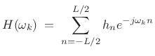
Let the FIR filter length be samples, with even, and suppose we'll initially design it to be centered about the time origin (``zero phase''). Then the frequency response is given on our frequency grid $\omega_k$ by

$\displaystyle H(\omega_k) \eqsp \sum_{n=-L/2}^{L/2} h_n e^{-j\omega_kn}$

(5.33)

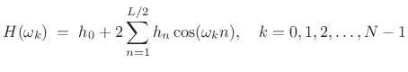
Enforcing even symmetry in the impulse response, i.e., $h_n = h_{-n}$ , gives a zero-phase FIR filter that we can later right-shift samples to make a causal, linear phase filter. In this case, the frequency response reduces to a sum of cosines:

$\displaystyle H( \omega_k ) \eqsp h_0 + 2\sum_{n=1}^{L/2} h_n \cos (\omega_k n), \quad k=0,1,2,\ldots, N-1$

(5.34)

or, in matrix form:

$\displaystyle \underbrace{\left[ \begin{array}{c} H(\omega_0) \\ H(\omega_1) \\ \vdots \\ H(\omega_{N-1}) \end{array} \right]}_{{\underline{d}}} = \underbrace{\left[ \begin{array}{ccccc} 1 & 2\cos(\omega_0) & \dots & 2\cos[\omega_0(L/2)] \\ 1 & 2\cos(\omega_1) & \dots & 2\cos[\omega_1(L/2)] \\ \vdots & \vdots & & \vdots \\ 1 & 2\cos(\omega_{N-1}) & \dots & 2\cos[\omega_{N-1}(L/2)] \end{array} \right]}_\mathbf{A} \underbrace{\left[ \begin{array}{c} h_0 \\ h_1 \\ \vdots \\ h_{L/2} \end{array} \right]}_{{\underline{h}}} \protect$

(5.35)

Recall from §3.13.8, that the Remez multiple exchange algorithm is based on this formulation internally. In that case, the left-hand-side includes the alternating error, and the frequency grid $\omega_k$ iteratively seeks the frequencies of maximum error--the so-called extremal frequencies.

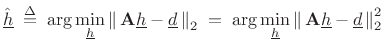
In matrix notation, our filter-design problem can be stated as (cf. §3.13.8)

$\displaystyle \min_{{\underline{h}}} \left\Vert \mathbf{A}{\underline{h}}-{\underline{d}}\right\Vert _2^2$

(5.36)

where these quantities are defined in (4.35). We can denote the optimal least-squares solution by

$\displaystyle {\underline{\hat{h}}}\isdefs \arg \min_{\underline{h}}\left\Vert\,\mathbf{A}{\underline{h}}-{\underline{d}}\,\right\Vert _2 \eqsp \arg \min_{\underline{h}}\left\Vert\,\mathbf{A}{\underline{h}}-{\underline{d}}\,\right\Vert _2^2$

(5.37)

To find ${\underline{\hat{h}}}$ , we need to minimize

$\displaystyle \left\Vert\,\mathbf{A}{\underline{h}}-{\underline{d}}\,\right\Vert _2^2$	$\displaystyle =$	$\displaystyle (\mathbf{A}{\underline{h}}-{\underline{d}})^T(\mathbf{A}{\underline{h}}-{\underline{d}})$
	$\displaystyle =$	$\displaystyle ({\underline{h}}^T\mathbf{A}^T-{\underline{d}}^T)(\mathbf{A}{\underline{h}}-{\underline{d}})$
	$\displaystyle =$	$\displaystyle {\underline{h}}^T\mathbf{A}^T\mathbf{A}{\underline{h}} -{\underline{h}}^T\mathbf{A}^T{\underline{d}} -{\underline{d}}^T\mathbf{A}{\underline{h}} +{\underline{d}}^T{\underline{d}} \protect$	(5.38)

This is a quadratic form in ${\underline{h}}$ . Therefore, it has a global minimum which we can find by setting the gradient to zero, and solving for ${\underline{h}}$ .^5.14Assuming all quantities are real, equating the gradient to zero yields the so-called normal equations

$\displaystyle \mathbf{A}^T\mathbf{A}{\underline{h}}\eqsp \mathbf{A}^T{\underline{d}}$

(5.39)

with solution

$\displaystyle \zbox {{\underline{\hat{h}}}\eqsp \left[(\mathbf{A}^T\mathbf{A})^{-1}\mathbf{A}^T\right]{\underline{d}}.}$

(5.40)

The matrix

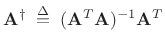$\displaystyle \mathbf{A}^\dagger \isdefs (\mathbf{A}^T\mathbf{A})^{-1}\mathbf{A}^T$

(5.41)

is known as the (Moore-Penrose) pseudo-inverse of the matrix $\mathbf {A}$ . It can be interpreted as an orthogonal projection matrix, projecting ${\underline{d}}$ onto the column-space of $\mathbf {A}$ [264], as we illustrate further in the next section.

Geometric Interpretation of Least Squares

Typically, the number of frequency constraints is much greater than the number of design variables (filter coefficients). In these cases, we have an overdetermined system of equations (more equations than unknowns). Therefore, we cannot generally satisfy all the equations, and are left with minimizing some error criterion to find the ``optimal compromise'' solution.

In the case of least-squares approximation, we are minimizing the Euclidean distance, which suggests the geometrical interpretation shown in Fig.4.19.

$\begin{psfrags} % latex2html id marker 14494\psfrag{Ax}{{\Large $\mathbf{A}{\underline{\hat{h}}}$}}\psfrag{b}{{\Large ${\underline{d}}$}}\psfrag{column}{{\Large column-space of $\mathbf{A}$}}\psfrag{space}{}\begin{figure}[htbp] \includegraphics[width=3in]{eps/lsq} \caption{Geometric interpretation of orthogonal projection of the vector ${\underline{d}}$\ onto the column-space of $\mathbf{A}$.} \end{figure} \end{psfrags}$
Thus, the desired vector ${\underline{d}}$ is the vector sum of its best least-squares approximation $\mathbf{A}{\underline{\hat{h}}}$ plus an orthogonal error :

$\displaystyle {\underline{d}}\eqsp \mathbf{A}{\underline{\hat{h}}}+ {\underline{e}}.$

(5.42)

In practice, the least-squares solution ${\underline{\hat{h}}}$ can be found by minimizing the sum of squared errors:

$\displaystyle \hbox{Minimize}_{\underline{h}}\Vert{\underline{e}}\Vert _2 \eqsp \Vert{\underline{d}}-\mathbf{A}{\underline{h}}\Vert _2$

(5.43)

Figure 4.19 suggests that the error vector ${\underline{d}}-\mathbf{A}{\underline{\hat{h}}}$ is orthogonal to the column space of the matrix $\mathbf {A}$ , hence it must be orthogonal to each column in $\mathbf {A}$ :

$\displaystyle \mathbf{A}^T({\underline{d}}-\mathbf{A}{\underline{\hat{h}}})\eqsp 0 \quad\Rightarrow\quad \mathbf{A}^T\mathbf{A}{\underline{\hat{h}}}\eqsp \mathbf{A}^T{\underline{d}}$

(5.44)

This is how the orthogonality principle can be used to derive the fact that the best least squares solution is given by

$\displaystyle {\underline{\hat{h}}}\eqsp (\mathbf{A}^T\mathbf{A})^{-1}\mathbf{A}^T {\underline{d}}\eqsp \mathbf{A}^\dagger {\underline{d}}$

(5.45)

In matlab, it is numerically superior to use ``h= A h'' as opposed to explicitly computing the pseudo-inverse as in ``h = pinv(A) * d''. For a discussion of numerical issues in matrix least-squares problems, see, e.g., [92].

We will return to least-squares optimality in §5.7.1 for the purpose of estimating the parameters of sinusoidal peaks in spectra.

Matlab Support for Least-Squares FIR Filter Design

Some of the available functions are as follows:

firls - least-squares linear-phase FIR filter design for piecewise constant desired amplitude responses -- also designs Hilbert transformers and differentiators
fircls - constrained least-squares linear-phase FIR filter design for piecewise constant desired amplitude responses -- constraints provide lower and upper bounds on the frequency response
fircls1 - constrained least-squares linear-phase FIR filter design for lowpass and highpass filters -- supports relative weighting of pass-band and stop-band error

For more information, type help firls and/or doc firls, etc., and refer to the ``See Also'' section of the documentation for pointers to more relevant functions.

Next Section:
Chebyshev FIR Design via Linear Programming
Previous Section:
Optimal Chebyshev FIR Filters