


Least Squares Sinusoidal Parameter Estimation
There are many ways to define ``optimal'' in signal modeling. Perhaps the most elementary case is least squares estimation. Every estimator tries to measure one or more parameters of some underlying signal model. In the case of sinusoidal parameter estimation, the simplest model consists of a single complex sinusoidal component in additive white noise:
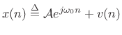
where
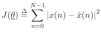
with respect to the parameter vector
![$\displaystyle \underline{\theta}\isdef \left[\begin{array}{c} A \\ [2pt] \phi \\ [2pt] \omega_0 \end{array}\right],$](http://www.dsprelated.com/josimages_new/sasp2/img1033.png) |
(6.34) |
where
 |
(6.35) |
Note that the error signal
Sinusoidal Amplitude Estimation
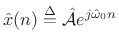
If the sinusoidal frequency ![]() and phase
and phase ![]() happen to be
known, we obtain a simple linear least squares problem for the
amplitude
happen to be
known, we obtain a simple linear least squares problem for the
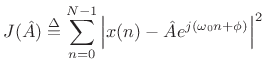
amplitude ![]() . That is, the error signal
. That is, the error signal
| (6.36) |
becomes linear in the unknown parameter
becomes a simple quadratic (parabola) over the real line.6.11 Quadratic forms in any number of dimensions are easy to minimize. For example, the ``bottom of the bowl'' can be reached in one step of Newton's method. From another point of view, the optimal parameter
Yet a third way to minimize (5.37) is the method taught in
elementary calculus: differentiate
![]() with respect to
with respect to ![]() , equate
it to zero, and solve for
, equate
it to zero, and solve for ![]() . In preparation for this, it is helpful to
write (5.37) as
. In preparation for this, it is helpful to
write (5.37) as
![\begin{eqnarray*}
J({\hat A}) &\isdef & \sum_{n=0}^{N-1}
\left[x(n)-{\hat A}e^{j(\omega_0 n+\phi)}\right]
\left[\overline{x(n)}-\overline{{\hat A}} e^{-j(\omega_0 n+\phi)}\right]\\
&=&
\sum_{n=0}^{N-1}
\left[
\left\vert x(n)\right\vert^2
-
x(n)\overline{{\hat A}} e^{-j(\omega_0 n+\phi)}
-
\overline{x(n)}{\hat A}e^{j(\omega_0 n+\phi)}
+
{\hat A}^2
\right]
\\
&=& \left\Vert\,x\,\right\Vert _2^2 - 2\mbox{re}\left\{\sum_{n=0}^{N-1} x(n)\overline{{\hat A}}
e^{-j(\omega_0 n+\phi)}\right\}
+ N {\hat A}^2.
\end{eqnarray*}](http://www.dsprelated.com/josimages_new/sasp2/img1045.png)
Differentiating with respect to ![]() and equating to zero yields
and equating to zero yields
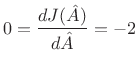 re re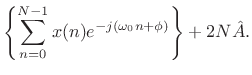 |
(6.38) |
Solving this for
 re
re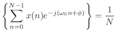 re
reThat is, the optimal least-squares amplitude estimate may be found by the following steps:
- Multiply the data
 by
by
 to zero the known phase
  .
.
- Take the DFT of the
 samples of
  , suitably zero padded to approximate the DTFT, and evaluate it at the known frequency
  .
.
- Discard any imaginary part since it can only contain noise, by (5.39).
- Divide by
to obtain a properly normalized coefficient of projection
[264] onto the sinusoid
(6.40)
Sinusoidal Amplitude and Phase Estimation
The form of the optimal estimator (5.39) immediately suggests the following generalization for the case of unknown amplitude and phase:
That is,
The orthogonality principle for linear least squares estimation states
that the projection error must be orthogonal to the model.
That is, if ![]() is our optimal signal model (viewed now as an
is our optimal signal model (viewed now as an
![]() -vector in
-vector in ![]() ), then we must have [264]
), then we must have [264]

Thus, the complex coefficient of projection of ![]() onto
onto
![]() is given by
is given by
 |
(6.42) |
The optimality of
 |
Sinusoidal Frequency Estimation
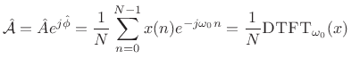
The form of the least-squares estimator (5.41) in the known-frequency case immediately suggests the following frequency estimator for the unknown-frequency case:
That is, the sinusoidal frequency estimate is defined as that frequency which maximizes the DTFT magnitude. Given this frequency, the least-squares sinusoidal amplitude and phase estimates are given by (5.41) evaluated at that frequency.
It can be shown [121] that (5.43) is in fact the optimal least-squares estimator for a single sinusoid in white noise. It is also the maximum likelihood estimator for a single sinusoid in Gaussian white noise, as discussed in the next section.
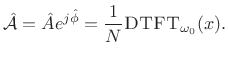
In summary,
In practice, of course, the DTFT is implemented as an interpolated FFT, as described in the previous sections (e.g., QIFFT method).
Next Section:
Maximum Likelihood Sinusoid Estimation
Previous Section:
Bias of Parabolic Peak Interpolation


