


White Noise
Definition:
To say that ![]() is a white noise means merely that
successive samples are uncorrelated:
is a white noise means merely that
successive samples are uncorrelated:
![$\displaystyle E\{v(n)v(n+m)\} = \left\{\begin{array}{ll} \sigma_v^2, & m=0 \\ [5pt] 0, & m\neq 0 \\ \end{array} \right. \isdef \sigma_v^2 \delta(m) \protect$](http://www.dsprelated.com/josimages_new/sasp2/img2676.png)
where
In other words, the autocorrelation function of white noise is an impulse at lag 0. Since the power spectral density is the Fourier transform of the autocorrelation function, the PSD of white noise is a constant. Therefore, all frequency components are equally present--hence the name ``white'' in analogy with white light (which consists of all colors in equal amounts).
Making White Noise with Dice
An example of a digital white noise generator is the sum of a pair of
dice minus 7. We must subtract 7 from the sum to make it zero
mean. (A nonzero mean can be regarded as a deterministic component at
dc, and is thus excluded from any pure noise signal for our purposes.)
For each roll of the dice, a number between
![]() and
and ![]() is generated. The numbers are distributed binomially between
is generated. The numbers are distributed binomially between ![]() and
and
![]() , but this has nothing to do with the whiteness of the number
sequence generated by successive rolls of the dice. The value of a
single die minus
, but this has nothing to do with the whiteness of the number
sequence generated by successive rolls of the dice. The value of a
single die minus ![]() would also generate a white noise sequence,
this time between
would also generate a white noise sequence,
this time between ![]() and
and ![]() and distributed with equal
probability over the six numbers
and distributed with equal
probability over the six numbers
![$\displaystyle \left[-\frac{5}{2}, -\frac{3}{2}, -\frac{1}{2}, \frac{1}{2}, \frac{3}{2}, \frac{5}{2}\right].$](http://www.dsprelated.com/josimages_new/sasp2/img2686.png) |
(C.27) |
To obtain a white noise sequence, all that matters is that the dice are sufficiently well shaken between rolls so that successive rolls produce independent random numbers.C.4
Independent Implies Uncorrelated
It can be shown that independent zero-mean random numbers are also uncorrelated, since, referring to (C.26),
![$\displaystyle E\{\overline{v(n)}v(n+m)\} = \left\{\begin{array}{ll} E\{\left\vert v(n)\right\vert^2\} = \sigma_v^2, & m=0 \\ [5pt] E\{\overline{v(n)}\}\cdot E\{v(n+m)\}=0, & m\neq 0 \\ \end{array} \right. \isdef \sigma_v^2 \delta(m)$](http://www.dsprelated.com/josimages_new/sasp2/img2689.png) |
(C.28) |
For Gaussian distributed random numbers, being uncorrelated also implies independence [201]. For related discussion illustrations, see §6.3.
Estimator Variance
As mentioned in §6.12, the pwelch function in Matlab
and Octave offer ``confidence intervals'' for an estimated power
spectral density (PSD). A confidence interval encloses the
true value with probability ![]() (the confidence level). For
example, if
(the confidence level). For
example, if ![]() , then the confidence level is
, then the confidence level is ![]() .
.
This section gives a first discussion of ``estimator variance,'' particularly the variance of sample means and sample variances for stationary stochastic processes.
Sample-Mean Variance
The simplest case to study first is the sample mean:
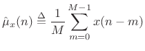 |
(C.29) |
Here we have defined the sample mean at time
| (C.30) |
or
 |
(C.31) |
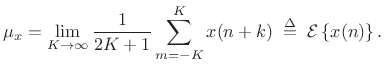
Now assume
Var![$\displaystyle \left\{x(n)\right\} \isdefs {\cal E}\left\{[x(n)-\mu_x]^2\right\} \eqsp {\cal E}\left\{x^2(n)\right\} \eqsp \sigma_x^2$](http://www.dsprelated.com/josimages_new/sasp2/img2697.png) |
(C.32) |
Then the variance of our sample-mean estimator
![]() can be calculated as follows:
can be calculated as follows:
![\begin{eqnarray*}
\mbox{Var}\left\{\hat{\mu}_x(n)\right\} &\isdef & {\cal E}\left\{\left[\hat{\mu}_x(n)-\mu_x \right]^2\right\}
\eqsp {\cal E}\left\{\hat{\mu}_x^2(n)\right\}\\
&=&{\cal E}\left\{\frac{1}{M}\sum_{m_1=0}^{M-1} x(n-m_1)\,
\frac{1}{M}\sum_{m_2=0}^{M-1} x(n-m_2)\right\}\\
&=&\frac{1}{M^2}\sum_{m_1=0}^{M-1}\sum_{m_2=0}^{M-1}
{\cal E}\left\{x(n-m_1) x(n-m_2)\right\}\\
&=&\frac{1}{M^2}\sum_{m_1=0}^{M-1}\sum_{m_2=0}^{M-1}
r_x(\vert m_1-m_2\vert)
\end{eqnarray*}](http://www.dsprelated.com/josimages_new/sasp2/img2699.png)
where we used the fact that the time-averaging operator
![]() is
linear, and
is
linear, and ![]() denotes the unbiased autocorrelation of
denotes the unbiased autocorrelation of ![]() .
If
.
If ![]() is white noise, then
is white noise, then
![]() , and we obtain
, and we obtain
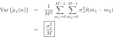
We have derived that the variance of the ![]() -sample running average of
a white-noise sequence
-sample running average of
a white-noise sequence ![]() is given by
is given by
![]() , where
, where
![]() denotes the variance of
denotes the variance of ![]() . We found that the
variance is inversely proportional to the number of samples used to
form the estimate. This is how averaging reduces variance in general:
When averaging
. We found that the
variance is inversely proportional to the number of samples used to
form the estimate. This is how averaging reduces variance in general:
When averaging ![]() independent (or merely uncorrelated) random
variables, the variance of the average is proportional to the variance
of each individual random variable divided by
independent (or merely uncorrelated) random
variables, the variance of the average is proportional to the variance
of each individual random variable divided by ![]() .
.
Sample-Variance Variance
Consider now the sample variance estimator
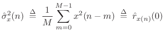 |
(C.33) |
where the mean is assumed to be
![$ {\cal E}\left\{[\hat{\sigma}_x^2(n)]^2\right\} = {\cal E}\left\{\hat{r}_{x(n)}^2(0)\right\} = \sigma_x^2$](http://www.dsprelated.com/josimages_new/sasp2/img2708.png) .
The variance of this estimator is then given by
.
The variance of this estimator is then given by
![\begin{eqnarray*}
\mbox{Var}\left\{\hat{\sigma}_x^2(n)\right\} &\isdef & {\cal E}\left\{[\hat{\sigma}_x^2(n)-\sigma_x^2]^2\right\}\\
&=& {\cal E}\left\{[\hat{\sigma}_x^2(n)]^2-\sigma_x^4\right\}
\end{eqnarray*}](http://www.dsprelated.com/josimages_new/sasp2/img2709.png)
where
![\begin{eqnarray*}
{\cal E}\left\{[\hat{\sigma}_x^2(n)]^2\right\} &=&
\frac{1}{M^2}\sum_{m_1=0}^{M-1}\sum_{m_1=0}^{M-1}{\cal E}\left\{x^2(n-m_1)x^2(n-m_2)\right\}\\
&=& \frac{1}{M^2}\sum_{m_1=0}^{M-1}\sum_{m_1=0}^{M-1}r_{x^2}(\vert m_1-m_2\vert)
\end{eqnarray*}](http://www.dsprelated.com/josimages_new/sasp2/img2710.png)
The autocorrelation of ![]() need not be simply related to that of
need not be simply related to that of
![]() . However, when
. However, when ![]() is assumed to be Gaussian white
noise, simple relations do exist. For example, when
is assumed to be Gaussian white
noise, simple relations do exist. For example, when
![]() ,
,
| (C.34) |
by the independence of
When ![]() is assumed to be Gaussian white noise, we have
is assumed to be Gaussian white noise, we have
![$\displaystyle {\cal E}\left\{x^2(n-m_1)x^2(n-m_2)\right\} = \left\{\begin{array}{ll} \sigma_x^4, & m_1\ne m_2 \\ [5pt] 3\sigma_x^4, & m_1=m_2 \\ \end{array} \right.$](http://www.dsprelated.com/josimages_new/sasp2/img2721.png) |
(C.35) |
so that the variance of our estimator for the variance of Gaussian white noise is
Var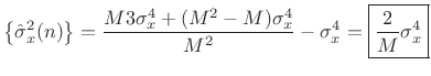 |
(C.36) |
Again we see that the variance of the estimator declines as
The same basic analysis as above can be used to estimate the variance of the sample autocorrelation estimates for each lag, and/or the variance of the power spectral density estimate at each frequency.
As mentioned above, to obtain a grounding in statistical signal processing, see references such as [201,121,95].
Next Section:
Gaussian Window and Transform
Previous Section:
Correlation Analysis


