


Relation of Smoothness to Roll-Off Rate
In §3.1.1, we found that the side lobes of
the rectangular-window transform ``roll off'' as ![]() . In this
section we show that this roll-off rate is due to the amplitude
discontinuity at the edges of the window. We also show that, more
generally, a discontinuity in the
. In this
section we show that this roll-off rate is due to the amplitude
discontinuity at the edges of the window. We also show that, more
generally, a discontinuity in the ![]() th derivative corresponds to a
roll-off rate of
th derivative corresponds to a
roll-off rate of
![]() .
.
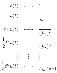
The Fourier transform of an impulse
![]() is simply
is simply
 |
(B.70) |
by the sifting property of the impulse under integration. This shows that an impulse consists of Fourier components at all frequencies in equal amounts. The roll-off rate is therefore zero in the Fourier transform of an impulse.
By the differentiation theorem for Fourier transforms
(§B.2), if
![]() , then
, then
| (B.71) |
where
 . Consequently, the integral
of
. Consequently, the integral
of  |
(B.72) |
The integral of the impulse is the unit step function:
![$\displaystyle \int_{-\infty}^t \delta(\tau)\,d\tau = u(t) \isdef \left\{\begin{array}{ll} 1, & t\geq0 \\ [5pt] 0, & t<0 \\ \end{array} \right.$](http://www.dsprelated.com/josimages_new/sasp2/img2578.png) |
(B.73) |
Therefore,B.4
 |
(B.74) |
Thus, the unit step function has a roll-off rate of
 |
(B.75) |
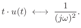
Integrating the unit step function gives a linear ramp function:
![$\displaystyle \int_{-\infty}^t u(\tau)d\tau = t \cdot u(t) = \left\{\begin{array}{ll} t, & t\geq0 \\ [5pt] 0, & t<0 \\ \end{array} \right..$](http://www.dsprelated.com/josimages_new/sasp2/img2586.png) |
(B.76) |
Applying the integration theorem again yields
 |
(B.77) |
Thus, the linear ramp has a roll-off rate of
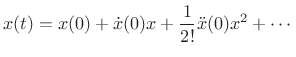
Now consider the Taylor series expansion of the function
![]() at
at
![]() :
:
 |
(B.78) |
The derivatives up to order
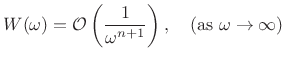
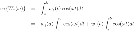
Theorem: (Riemann Lemma):
If the derivatives up to order ![]() of the function
of the function ![]() exist and
are of bounded variation (defined below), then its Fourier Transform
exist and
are of bounded variation (defined below), then its Fourier Transform
![]() is asymptotically of orderB.5
is asymptotically of orderB.5
![]() , i.e.,
, i.e.,
 |
(B.79) |
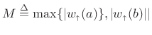
Proof: Following [202, p. 95], let
| (B.80) |
denote its decomposition into a nondecreasing part
Since
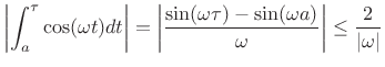 |
(B.82) |
we conclude
 |
(B.83) |
where
 , which is finite since
 |
(B.84) |
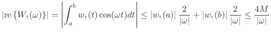
If in addition the derivative
![]() is bounded on
is bounded on ![]() , then
the above gives that its transform
, then
the above gives that its transform
![]() is
asymptotically of order
is
asymptotically of order ![]() , so that
, so that
![]() . Repeating this argument, if the first
. Repeating this argument, if the first ![]() derivatives exist and are of bounded variation on
derivatives exist and are of bounded variation on ![]() , we have
, we have
![]() .
.
![]()
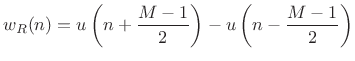
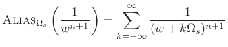
Since spectrum-analysis windows ![]() are often obtained by
sampling continuous time-limited functions
are often obtained by
sampling continuous time-limited functions ![]() , we
normally see these asymptotic roll-off rates in aliased
form, e.g.,
, we
normally see these asymptotic roll-off rates in aliased
form, e.g.,
 |
(B.85) |
where
In summary, we have the following Fourier rule-of-thumb:
| (B.86) |
This is also
To apply this result to estimating FFT window roll-off rate (as in Chapter 3), we normally only need to look at the window's endpoints. The interior of the window is usually differentiable of all orders. For discrete-time windows, the roll-off rate ``slows down'' at high frequencies due to aliasing.
Next Section:
Random Variables & Stochastic Processes
Previous Section:
The Uncertainty Principle


