


The Running-Sum Lowpass Filter
Perhaps the simplest FIR lowpass filter is the so-called
running-sum lowpass filter [175]. The impulse
response of the length ![]() running-sum lowpass filter is given by
running-sum lowpass filter is given by
![$\displaystyle h(n) \isdef \left\{\begin{array}{ll} 1, & n=0,1,2,...,N-1 \\ [5pt] 0, & \hbox{otherwise.} \\ \end{array} \right. \protect$](http://www.dsprelated.com/josimages_new/sasp2/img1568.png)
Figure 9.10 depicts the generic operation of filtering ![]() by
by ![]() to produce
to produce ![]() , where
, where ![]() is the impulse response of the
filter. The output signal is given by the convolution of
is the impulse response of the
filter. The output signal is given by the convolution of ![]() and
and ![]() :
:
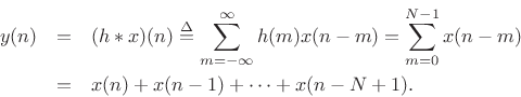
In this form, it is clear why the filter (9.5) is called
``running sum'' filter. Dividing it by ![]() , it becomes a ``moving
average'' filter, averaging the most recent
, it becomes a ``moving
average'' filter, averaging the most recent ![]() input samples.
input samples.
The transfer function of the running-sum filter is given by [263]
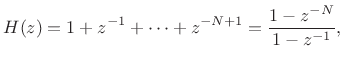 |
(10.6) |
so that its frequency response is
![\begin{eqnarray*}
H(e^{j\omega}) &=& \frac{1-e^{-j\omega N}}{1-e^{-j\omega }}
= \frac{e^{-j\omega N/2}}{e^{-j\omega /2}}
\frac{\sin(\omega N/2)}{\sin(\omega /2)}\\ [10pt]
&\isdef &
Ne^{-j\omega(N-1)/2} \hbox{asinc}_N(\omega ).
\end{eqnarray*}](http://www.dsprelated.com/josimages_new/sasp2/img1572.png)
Recall that the term
![]() is a linear phase
term corresponding to a delay of
is a linear phase
term corresponding to a delay of ![]() samples (half of the FIR
filter order). This arises because we defined the running-sum lowpass
filter as a causal, linear phase filter.
samples (half of the FIR
filter order). This arises because we defined the running-sum lowpass
filter as a causal, linear phase filter.
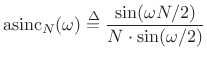
We encountered the ``aliased sinc function''
 |
(10.7) |
previously in Chapter 5 (§3.1.2) and elsewhere as the Fourier transform (DTFT) of a sampled rectangular pulse (or rectangular window).
Note that the dc gain of the length ![]() running sum filter is
running sum filter is ![]() . We
could use a moving average instead of a running sum (
. We
could use a moving average instead of a running sum (
![]() ) to obtain unity dc gain.
) to obtain unity dc gain.
![\includegraphics[width=4in]{eps/sincabs}](http://www.dsprelated.com/josimages_new/sasp2/img1577.png)
Figure 9.11 shows the amplitude response of the running-sum
lowpass filter for length ![]() . The gain at dc is
. The gain at dc is ![]() , and nulls
occur at
, and nulls
occur at
![]() and
and ![]() . These nulls occur
at the sinusoidal frequencies having respectively one and two periods
under the 5-sample ``rectangular window''. (Three periods would need
at least
. These nulls occur
at the sinusoidal frequencies having respectively one and two periods
under the 5-sample ``rectangular window''. (Three periods would need
at least
![]() samples, so
samples, so ![]() doesn't ``fit''.) Since
the pass-band about dc is not flat, it is better to call this a
``dc-pass filter'' rather than a ``lowpass filter.'' We could also
call it a dc sampling filter.10.1
doesn't ``fit''.) Since
the pass-band about dc is not flat, it is better to call this a
``dc-pass filter'' rather than a ``lowpass filter.'' We could also
call it a dc sampling filter.10.1
Next Section:
Modulation by a Complex Sinusoid
Previous Section:
Computational Examples in Matlab


