


An Efficient Linear Interpolation Scheme
This blog presents a computationally-efficient linear interpolation trick that requires at most one multiply per output sample.
Background: Linear Interpolation
Looking at Figure 1(a) let's assume we have two points, [x(0),y(0)] and [x(1),y(1)], and we want to compute the value y, on the line joining those two points, associated with the value x.
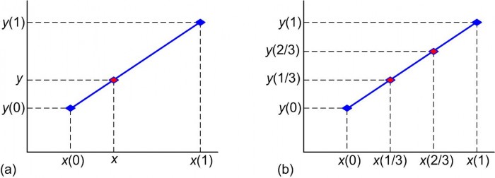
Figure 1: Linear interpolation: given x, x(0), x(1), y(0), and y(1), compute the value of y.
Equating the slopes of line segments on the blue line in Figure 1(a) we can write:
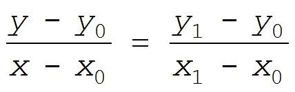 . (1)
. (1)
Solving Eq. (1) for y gives us:
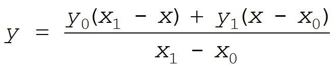 . (2)
. (2)
Equation (2) requires four additions, two multiplications, and one division to compute a single y value. As in Figure 1(b) to compute, say, two different intermediate y values on the blue line requires us to evaluate Eq. (2) twice.
Linear Interpolation With Time-Domain Periodic Samples
DSP folks, when processing periodically sampled time-domain x(k) sequences, have a better scheme for linear interpolation. In that scenario, for example, the z-domain transfer function of an L = 3 linear interpolator is:
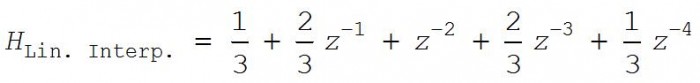 (3)
(3)
implemented in a tapped-delay line structure as shown in Figure 2. The "↑L" upsample process means insert L–1 zero-valued samples in-between each sample of the x(k) input sequence.
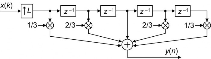
Figure 2: L = 3 DSP linear interpolator block diagram.
The traditional Figure 2 interpolation method requires 2L-2 multiplies and 2L-2 additions per output sample. The following proposed linear interpolation is more computationally efficient.
Proposed Efficient Linear Interpolation
Our efficient linear interpolator is the simple network shown in Figure 3. That mysterious block labeled 'Zero-Order Hold' is merely the operation where each u(k) input sample is repeated L–1 times. For example, if L = 3 and the input to the Zero-Order Hold operation is {1,-4,3}, the output of the process is {1,1,1,-4,-4,-4,3,3,3}.
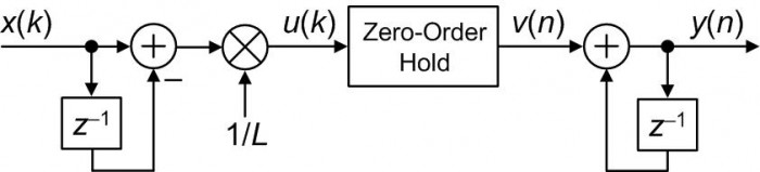
Figure 3: Proposed linear interpolation block diagram.
The example sequences in Figure 4 highlight the operation of the proposed Figure 3 linear interpolator.
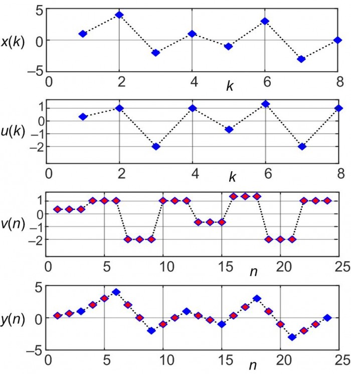
Figure 4: Proposed linear interpolation example sequences when L = 3.
The important details to notice in Figure 4 are:
• The v(n) sequence is simply the u(k) sequence with each u(k) sample repeated L-1 = 2 times (zero-order hold)
• The x(k) input samples are preserved in the y(n) output sequence
• The transient response of our proposed interpolator is L-1 samples, so the first valid output sample is the L-1 = 2nd y(n) sample
• If we're able to set L to an integer power of two then, happily, the 1/L multiplication can be implemented with a binary arithmetic right shift by log2(L) bits yielding a multiplierless linear interpolator
• If an interpolator output/input gain of L is acceptable, the 1/L multiplication can be eliminated.
Fixed-Point Arithmetic Implementation
When implemented in fixed-point two's complement arithmetic, the 1/L multiply in Figure 3 induces significant (and unpredictable) quantization distortion in the y(n) output, particularly when the x(k) input is low in frequency or small in amplitude. We can drastically reduce that distortion by moving the 1/L multiplication to be the final operation as shown in Figure 5.
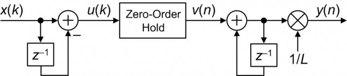
Figure 5: Fixed-point arithmetic implementation of the proposed linear interpolator.
When using two's complement arithmetic, if the x(k) input samples are N bits in width then the bit width of the accumulator register used in the first adder must be N+1 bits in width.
We must ensure that the bit width of the accumulator register used in the second adder be large enough to accommodate a gain of L from the x(k) input to the output of the second adder.
As with the Figure 3 implementation, if the value L in Figure 5 is an integer power of two then a binary right shift can eliminate the final 1/L multiplication. And again, if an interpolator gain of L is acceptable then no 1/L scaling need be performed in Figure 5.
Conclusions
We've introduced efficient floating-point (Figure 3) and fixed-point (Figure 5) linear interpolators. Their computational workloads are compared in Appendix A.
The experienced reader might now say, "Ah, while those networks are computationally simple, linear interpolation is certainly not the most accurate method of interpolation, particularly for large interpolation factors." Rocky Balboa would reply with, "This is very true. But if interpolation is being done in multiple stages, using these efficient interpolators as the final stage at the highest data rate (when the signal samples are already close together) will introduce only a small interpolation error."

Appendix A: Computational Workload Comparison
Table A-1 compares the arithmetic workload of the above linear interpolation by L methods, measured in computations per output sample.
Table A-1: Arithmetic computations per output sample for linear interpolation by L.
| | Additions | Multiplies | Divides |
| General linear interpolation [Eq. (2)] | 4L | 2L | L |
| Periodically sampled input [Eq. (3)] | 2L-2 | 2L-2 | -- |
| Proposed Interpolation (Gain = 1, fixed-point) [Figure 5] | L + 1/L | L | -- |
| Proposed Interpolation (Gain = 1, floating-point) [Figure 3] | L + 1/L | 1/L | -- |
| Proposed Interpolation (Gain = L, fixed- or floating-point) | L + 1/L | -- | -- |
- Comments
- Write a Comment Select to add a comment

Hi Rick,
Thanks for the article. Correct me please if I am wrong
a) For a time sequence y(0) ~ y(n) a new y is just half of diff of two adjacent samples relative to last sample
b) For other functions of y i.e. y = f(x) and assuming we want new value of y anywhere along the line then how would figure 5 get L and where in the design is the location of y entered.
Regards
Kaz

Hi Kaz.
Please forgive me but I don't understand your comment (a). Looking at my Figure 4 can you tell me which of the x(k), u(k), v(n), or y(n) sequences you are referring to?
Regarding your comment (b), I am puzzled. I don't know what you mean by "other functions." In the Figure 5 linear interpolator the variable 'L' is used to determine the multiplier coefficient 1/L. And we don't "enter" (i.e., specify) any sort of 'y' variable. The 'y(n)' sequence is the computed, periodically-spaced-in-time, interpolator output sequence.
Hi Rick,
Sorry I think there is a problem in your design but I didn't express my observation in a relevant sense.
That problem can be reasoned as follows:
Assume L = 5 i.e. I want to inject four new samples in between x1 & x2 input samples.
Common sense tells me that the interval between x1 & x2 has to be divided by 5 then 1/5 of that interval accumulated four times and added to x1, right?
so yes you are accumulating (x2-x1) then dividing by L but you must add x1 to the accumulated 1/5ths for each new sample then reset accumulator once you arrive at x2.
Your design just gets (x2-x1)/L then accumulates that on itself nonstop.
I really don't see how is it going to work. Your help appreciated.
Hi Rick again,
I just run a model and realised your design works if and only if the input has one zero initially. Otherwise the accum gets out of control(creates dc offset). It could be my model?
Here is my model
%%%%%%%%%%%%%%%%%%%%%%%%%%%%%%%%
L = 9; %interpolation factor
x = randn(1,1024); %randm input
x(1) = 0;
u = zeros(1,length(x));
for i = 2:length(x)
u(i) = x(i) - x(i-1); %subtractor
end
v = zeros(1,length(x)*L);
for i = 1:L
v(i:L:end) = u/L; %repeat samples L-1 and divide
end
y = zeros(1,length(v));
for i = 2:length(v)
y(i) = v(i) + y(i-1); %accumulator
end
%display input/output
x_rpt = zeros(1,length(x)*L);
for i = 1:L
x_rpt(i:L:end) = x;
end
plot(x_rpt,'.-');hold;
plot(y,'.r--');
%%%%%%%%%%%%%%%%%%%%%%%%%%%%%%%%%%%
Regards
Kaz
Hi Kaz. My compliments to you for your enthusiasm! After some effort I now see what's happening in your code. Try this:
[1] Set you input 'x' sequence to my Figure 4's 'x(k)' using:
x = [1, 4, -2, 1, -1, 3, -3, 0];
[2] Replace your three-line 'for loop' commands that compute your 'u' variable with the single command:
u = filter([1, -1], 1, x);
[3] Replace your three-line 'for loop' commands that compute your 'y' variable with the single command:
y = filter(1, [1, -1], v);
After making those three changes your code produces a correct 'y' sequence that's equal to my Figure 4's 'y(k)'. And there's no need to worry about having any initial zero-valued samples at the beginning of the 'x' input sequence.
Happy New Year Kaz.
Thanks Rick,
That's it. I personally prefer using the "filter" function for all of my fir or iir models as it is fast and accurate but just went down to direct slow loops this time.
The bug in my two for loops was due to my assumption that hardware(fpga in my mind) starts as zeros on registers but math does not see it that way and does not recognize that as sample.
so now I initialised u as u(1) = x(1) and initialised y(1) = v(1) and it behaved.
good lesson in modelling for me.
Regards
Kaz
%%%%%%%%%%%%%%%%%%%%%%%%%%%%%
clear all; clc;
L = 7; %interpolation factor
x = randn(1,1024); %randm input
u = zeros(1,length(x));
u(1) = x(1);
for i = 2:length(x)
u(i) = x(i) - x(i-1); %subtractor
end
v = zeros(1,length(x)*L);
for i = 1:L
v(i:L:end) = u/L; %repeat samples L-1 and divide
end
y = zeros(1,length(v));
y(1) = v(1);
for i = 2:length(v)
y(i) = v(i) + y(i-1); %accumulator
end
%display input/output
x_rpt = zeros(1,length(x)*L);
for i = 1:L
x_rpt(i:L:end) = x;
end
plot(x_rpt,'.-');hold;
plot(y,'.r--');
%%%%%%%%%%%%%%%%%%%%%%%%%%%%%%%%
The alternative is to add a zero to input stream instead of forcing sample 1 to zero and we do that a lot at work as it makes sense with fpga mindset
You write:
«The traditional Figure 2 interpolation method requires 2L-2 multiplies and 2L additions per output sample.«
Yet I count only 2L-1 adds in your figure.
Further:
It seems fair to use a standard polyphase/commutator structure as a baseline (avoid multiplying by zero). In that case, the three phases are:
y1 = (1/3)*x(n) + (2/3)*x(n-1)
y2 = (2/3)*x(n) + (1/3)*x(n-1)
y3 = x(n)
Rewrite as:
x2(n) = x(n)*(1/3)
y1 = x2(n) + x2(n-1) + x2(n-1)
y2 = x2(n) + x2(n) + x2(n-1)
y3 = x(n)
Thus we have 1/L mult and (L-1)*(L-1)/L adds per output sample. For L=3, this turns out to be The exact same numbers as your proposal.
Your topology seems to have similarities with CIC filters, yet not use wrap-around arithmetics. Any comments on that?
Regards
Knut Ing
Hi Knut Ing.
[1] You’re right! My text “2L additions per output sample” for Figure 2 was typographical error. It should be “2L–2 additions per output sample.” Thanks for pointing that error out to me Knut.
[2] Regarding your comment about a polyphase filter, there are no ‘multiply by zero’ operations in my Figure 3 network, but your comment is definitely interesting. I look forward to studying your polyphase idea in more detail.
[3] I was waiting to see if someone commented on the similarity of my Figure 3 network and CIC filters. As it turns out, my Figure 3 network is equivalent to a two-stage ‘interpolate-by-L’ CIC filter where the CIC filter’s second comb and first integrator are replaced by the ‘Zero-Order Hold’ operation. (The Figure 3 network was first shown to me years ago by digital filter expert Ricardo Losada of Mathworks Inc.) In any case, I did mention the use of two’s complement arithmetic (which exhibits modular wraparound behavior) in the text just before and just after my Figure 5.
Thanks for an enlightening post and follow-up discussion.
>>2] Regarding your comment about a polyphase filter, there are no ‘multiply by zero’ operations in my Figure 3 network
Sorry, I should have been more explicit. My comment was directed towards the Figure 2 topology. My understanding is that you are offering this as a "baseline" upon which your proposal (of Figure 3) appears to offer significant improvement.
My comment is that the topology of Figure 2, while consistent with how integer/fractional resampling is presented in dsp101 books seems to not be "state-of-the-art" in that it implements an upsampler as a chain of zero-stuffing and LTI filter. It has been known, I believe, since at least the publishing of Crochiere and Rabiner in the early 1980s, possibly Farrow in 1988 and nicely presented by Vaidyanathan in 1993 that Multirate/polyphase/commutator type topologies does this more efficiently (in particular for large ratios, L).
>> [3] I was waiting to see if someone commented on the similarity of my Figure 3 network and CIC filters... In any case, I did mention the use of two’s complement arithmetic (which exhibits modular wraparound behavior) in the text just before and just after my Figure 5.
I have been trying to wrap my head around CIC since discovering them relatively recently. Enough to notice that there is at least some superficial similarity to your Figure 3, but not enough to really understand what is going on.
My understanding is that CIC can _only_ be implemented by wrap-around integer arithmetic, while your structure can be perfectly well implemented using floating-point?
regards
Knut Inge
Figure 3 design is identical to one stage CIC interpolator with one delay unit comb followed by an integrator. The only difference is that it repeats samples L-1 times between comb and integrator while CIC inserts L-1 zeros. I view it as a subset of CIC.
Kaz
Hi kaz. Sorry, I should have been more specific in my previous Jan. 5th reply. What I mean to say is that the following two networks are equivalent.
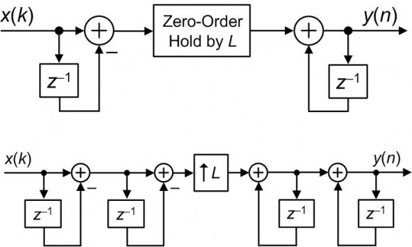
An explanation of my above claim can be found in the article: Ricardo Losada and Richard Lyons, "Reducing CIC Filter Complexity", IEEE Signal Processing Magazine, DSP Tips & Tricks column, Vol. 23, No. 4, July 2006.
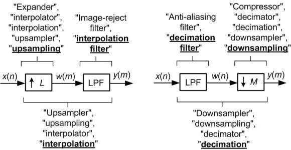
So trying to summarize:
1. "A Zero-order Hold by L" element is equivalent to upsampling by L (zero stuffing) followed by a boxcar FIR filter
2. By adding comb/integrator stages to the CIC topology, one goes from a boxcar filter, to a triangular filter, and so on. This seems similar to constructing B-splines from convolving rectangular functions with itself?
http://www.chebfun.org/examples/approx/BSplineConv...
3. The zero-order-hold presented in the article in Figure 3 can be seen as an efficient implementation of CIC (reduce the number of stages by 1)
4. The topology presented in the article can be implemented using floating-point, while: "a FIR filter can use fixed or floating point math, a CIC filter uses only fixed point math."
Hi Knut. That wiki page claiming that a CIC filter uses only fixed point math (the wiki
author's Reference [2]) is incorrect. If you read Hogenaurer's original
paper, you'll see that his analysis of binary register growth within
multistage CIC filters is based on the assumption that two's complement math is used. There is no restriction that two's complement math must be used.
Also, the first sentence on that wiki page is incorrect. That sentence states that a CIC filter is an FIR filter "combined with an interpolator". Actually, when the FIR filter is combined with upsampling (zero-stuffing) the combination becomes an interpolator.
The terminology used in the literature of 'sample rate change' is very inconsistent. I describe that inconsistency in Chapter 10 of my "Understanding DSP book as:
Hi Rick,
Thanks, I checked those two designs posted on Jan 6, using my CIC matlab model and can confirm your above statement that they are functionally same.
Kaz
Hi kaz. Great. I'm glad to hear that.
Hi Knut. You are correct. Polyphase filtering is by far the most efficient method for performing a sample rate change on a discrete signal. I believe that polyphase filtering is the second greatest innovation in the entire field of digital filtering! As far as I can tell polyphase filtering was introduced to the world by:
Bellanger, M. et al, "Digital Filtering by Polyphase Network: Application to Sample-Rate Alteration and Filter Banks," IEEE Trans. on Acoust. Speech, and Signal Proc., Vol. ASSP‑24, No. 2, April 1974.
As for CIC filters, they too can be implemented with floating-point arithmetic. But they're normally used in very high-speed digital communications systems with fixed-point hardware using two's complement arithmetic. As of a few years ago CIC filters were "built-in" the following commercial integrated circuits:
* Intersil's (Harris)
-HSP50110 'Digital Quadrature Tuner' has three-stage CICs,
-HSP50214 'Programmable Downconverter' has five-stage CICs,
* Texas Instruments (Graychip)
--GC4014 'Quad Digital Downconverter' has a four-stage CIC,
--GC408114 'Quad Digital Upconverter' has a four-stage CIC,
* Analog Devices' AD9857 'Quad Digital Upconverter' has a five-stage CIC.
CICs are fascinating digital filters. At first they appear rather simple, but the more you learn about their implementation in sample rate change applications the more you learn about the subtleties of their behavior. There have been a huge number of published DSP articles involving CIC filters.
Knut, there's even a way to implement CIC filters that contain no integrators. I'm not joking! Information on that weird idea can be found in the article: Ricardo Losada and Richard Lyons, "Reducing CIC Filter Complexity", IEEE Signal Processing Magazine, DSP Tips & Tricks column, Vol. 23, No. 4, July 2006.Hey, I remember those Harris and Graychip IC's! We used some of the Harris parts back in the 1990's at a now-defunct startup company in a satellite phone system earth station. Before that, I used Raytheon Semiconductor (product line bought from TRW, now part of Northrop-Grumman, of course) half-band filters to ease analog anti-aliasing and reconstruction filter specs in a digital video system. Can you tell I'm a hardware jock?! Now I'm at a different Raytheon myself, and Raytheon Semiconductor no longer exists, 'cause we're a Frankenstein's monster made up of the original Raytheon, Hughes, E-Systems, and TI Defense.
I'm going to have to look up those Losada and Lyons papers. They both have the initials R.L. Too bad Ricardo doesn't have the last name Leon...
Thanks, Rick, Kaz, et al., I'm always learning something good from you guys! :>
Hi,
Always fun to play with integrators :)
Two observations:
1) the equivalence between Rick's proposed circuit with zero order hold and the '2nd' order CIC filter block diagram is the same optimization that one can do when designing a decimating CIC filter: the first differentiator after the rate-change block can be removed completely if the last integrator is reset at the low rate. Those two optimization are the dual of each other.
2) Using those filters (either the standard CIC or Rick's proposal) in an interpolating context is EXTREMELY risky as the filter only works fine as long as it properly comes out of reset, and that nothing bad ever happens to the integrator. You can see that the integrator is being fed with the difference between new input samples, and simply runs in an open loop matter. It will never clear. It is better practice to 'force' the integrator to the new input value every N samples so that the filter is guaranteed to track the input no matter what happens.
Dave
Hi Dave,
Agreed and in FPGA platform I will prefer not to depend on that single initial state but this is matter of design failure rather than platform failure except for some critical applications. I know there are plenty designs around that depend on single initial state to do various tasks such as some ips, ADCs and inhouse modules.
Kaz
Hi gretzteam. Darn, I'm not able to understand your paragraph 2). Can you tell me what the phrase "it properly comes out of reset" means? Also, I don't understand what "nothing bad ever happens to the integrator" means.
Hi Rick,
My comments apply more to hardware implementation in RTL for ASIC or FPGA.
All I'm saying is that this structure only works if it was started properly; the initial state matters, forever...To illustrate this, imagine that the filter is running fine and you set the integrator to some random value, say 100, at one cycle. That 'error' will stick forever and will never flush out! Since a linear interpolator is an FIR filter, this is not the behavior one would expect (errors should flush out after at most the length of the impulse response...).
A more likely scenario is if the filter can be enabled/disabled. Typically this is implemented as an 'enable' signal going to all the zm1 block in the diagram, disabling the clock (but keeping their value). When the filter is resumed later on, the integrator starts from its 'old' value, while the input is probably something completely different. That is what I mean by 'coming out of reset properly'.
Other scenarios could be quantization error buildup (unlikely but would happen if one doesn't keep all the bits coming out of the differentiator), timing error etc...
All this can be avoided by realizing that every L cycles, the integrator is equal to the previous input sample (linear interpolation goes through the input data points). Every L cycles, you can set the integrator to the previous input value, adding a multiplexer to the implementation (but saving an add operation!).
All of this is unlikely but makes an IC designer sleep better at night.
Dave
Hi Dave. Thanks for your additional explanation!!
Ah, I like that hardware talk! Thanks, Dave.

Thank you for the article,
How can I make a similar comparison as you did in Appendix A to compare the complexity of some of the methods that I have used?
Thank you in advance
Hello DanielFZL. If I understand your question, my answer is as follows:
Draw a block diagram of some "method" you used showing the arithmetic processing (multipliers, adders, etc.). Then for each input data sample determine the number of multiplications, the number of additions, and the number of divide operations performed to compute a single output sample.
To post reply to a comment, click on the 'reply' button attached to each comment. To post a new comment (not a reply to a comment) check out the 'Write a Comment' tab at the top of the comments.
Please login (on the right) if you already have an account on this platform.
Otherwise, please use this form to register (free) an join one of the largest online community for Electrical/Embedded/DSP/FPGA/ML engineers:


