Design IIR Highpass Filters

• Matlab
• Tutorials

This post is the fourth in a series of tutorials on IIR Butterworth filter design.  So far we covered lowpass [1], bandpass [2], and band-reject [3] filters; now we’ll design highpass filters.  The general approach, as before, has six steps:

1. Find the poles of a lowpass analog prototype filter with Ω_c = 1 rad/s.
2. Given the -3 dB frequency of the digital highpass filter, find the corresponding frequency of the analog highpass filter (pre-warping).
3. Transform the analog lowpass poles to analog highpass poles.
4. Transform the poles from the s-plane to the z-plane, using the bilinear transform.
5. Add N zeros at z= 1, where N is the filter order.
6. Convert poles and zeros to polynomials with coefficients a_n and b_n.

This article is available in PDF format for easy printing.

The detailed design procedure follows.  Recall from the previous posts that F is continuous (analog) frequency in Hz and Ω is continuous radian frequency.  A Matlab function hp_synth that performs the filter synthesis is provided in the Appendix.  Note that hp_synth(N,fc,fs) gives the same results as the Matlab function butter(N,2*fc/fs,’high’).

1.  Poles of the analog lowpass prototype filter.  For a Butterworth filter of order N with Ω_c = 1 rad/s, the poles are given by [4, 5]:

$$p'_{ak}= -sin(\theta)+jcos(\theta)$$

where $$\theta=\frac{(2k-1)\pi}{2N},\quad k=1:N$$

Here we use a prime superscript on p to distinguish the lowpass prototype poles from the yet to be calculated highpass poles.

2.  Given the -3 dB discrete frequency f_c of the digital highpass filter, find the corresponding frequency of the analog highpass filter.  As before, we’ll adjust (pre-warp) the analog frequency to take the nonlinearity of the bilinear transform into account:

$$F_c=\frac{f_s}{\pi}tan\left(\frac{\pi f_c}{f_s}\right)$$

3.  Transform the normalized analog lowpass poles to analog highpass poles.  For each lowpass pole p_a’, we get the highpass pole [6, 7]:

$$p_a=2\pi F_c/p'_a$$

4.  Transform the poles from the s-plane to the z-plane, using the bilinear transform [1]:  

$$p_k=\frac{1+p_{ak}/(2f_s)}{1-p_{ak}/(2f_s)},\quad k=1:N$$

5.  Add N zeros at z= 1.  The N^th-order highpass filter has N zeros at ω= 0, or z= exp(j0) = 1.  We can now write H(z) as:

$$H(z)=K\frac{(z-1)^N}{(z-p_1)(z-p_2)...(z-p_{N})}\qquad(1)$$

In hp_synth, we represent the N zeros at +1 as a vector:

q= ones(1,N)

6.  Convert poles and zeros to polynomials with coefficients a_n and b_n.  If we expand the numerator and denominator of equation 1 and divide numerator and denominator by z^N, we get polynomials in z^-n:

$$H(z)=K\frac{b_0+b_1z^{-1}+...+b_Nz^{-N}}{1+a_1z^{-1}+...+a_Nz^{-N}}\qquad(2)$$

The Matlab code to perform the expansion is:

a= poly(p)
a= real(a)
b= poly(q)

Given that H(z) is highpass, we want H(z) to have a gain of 1 at f = f_s/2, that is, at ω= π.  At ω= π, z = exp(jπ) = -1.  Referring to equation 2, we then have gain at ω= π of:

$$H(z=-1)=1=K\frac{\sum_{m=0}^N(-1)^m*b_m}{\sum_{m=0}^N(-1)^m*a_m}$$

So we have:

$$K= \frac{\sum_{m=0}^N(-1)^m*a_m}{\sum_{m=0}^N(-1)^m*b_m}$$

Example

Here is an example function call for a 5^th order highpass filter:

   N= 5;           % filter order
   fc= 40;         % Hz -3 dB frequency
   fs= 100;        % Hz  sample frequency
   [b,a]= hp_synth(N,fc,fs)
      b =    0.0013   -0.0064    0.0128   -0.0128    0.0064   -0.0013
      a =    1.0000    2.9754    3.8060    2.5453    0.8811    0.1254

To find the frequency response:

   [h,f]= freqz(b,a,512,fs);
   H= 20*log10(abs(h));

The resulting response is shown in Figure 1, along with the responses for N= 2, 3, and 7.  The pole-zero plot in the z-plane is shown in Figure 2.  

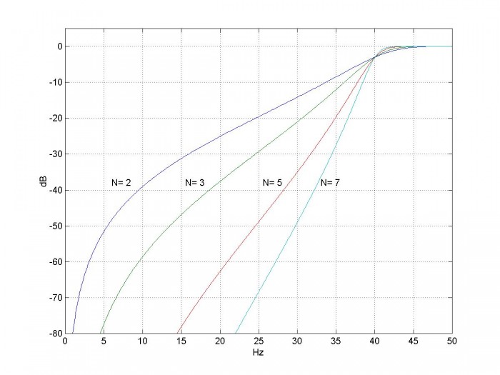
Figure 1.  Magnitude Response of Butterworth highpass filters for various filter orders.

                  f_c = 40 Hz and f_s = 100 Hz.

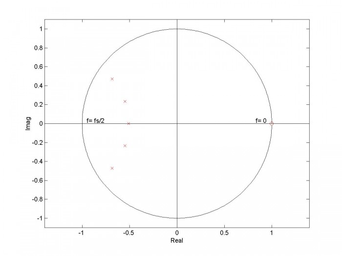
Figure 2.  Pole-zero plot of 5^th order Butterworth highpass filter.  f_c = 40 Hz and f_s = 100 Hz.

                   Zero at z= 1 is 5^th order.

References

1.  Robertson, Neil , “Design IIR Butterworth Filters Using 12 Lines of Code”, Dec 2017 https://www.dsprelated.com/showarticle/1119.php  

2.  Robertson, Neil , “Design IIR Bandpass Filters”, Jan 2017 https://www.dsprelated.com/showarticle/1128.php 

3.  Robertson, Neil , “Design IIR Band-Reject Filters”, Jan 2017 https://www.dsprelated.com/showarticle/1131.php

4.  Williams, Arthur B. and Taylor, Fred J., Electronic Filter Design Handbook, 3^rd Ed., McGraw-Hill, 1995, section 2.3

5.  Analog Devices Mini Tutorial MT-224, 2012 http://www.analog.com/media/en/training-seminars/tutorials/MT-224.pdf

6.  Blinchikoff, Herman J., and Zverev,Anatol I., Filtering in the Time and Frequency Domains, Wiley, 1976, section 4.3.

7.  Nagendra Krishnapura , “E4215: Analog Filter Synthesis and Design Frequency Transformation”,  4 Mar. 2003  http://www.ee.iitm.ac.in/~nagendra/E4215/2003/handouts/freq_transformation.pdf

Neil Robertson                  February, 2018

Appendix   Matlab Function hp_synth.m

This program is provided as-is without any guarantees or warranty.  The author is not responsible for any damage or losses of any kind caused by the use or misuse of the program.

% hp_synth.m    1/30/18 Neil Robertson
% Find the coefficients of an IIR Butterworth highpass filter using bilinear transform.
%
% N= filter order
% fc= -3 dB frequency in Hz
% fs= sample frequency in Hz
% b = numerator coefficients of digital filter
% a = denominator coefficients of digital filter
%
function [b,a]= hp_synth(N,fc,fs);
if fc>=fs/2;
   error('fc must be less than fs/2')
end
% I.  Find poles of normalized analog lowpass filter
k= 1:N;
theta= (2*k -1)*pi/(2*N);
p_lp= -sin(theta) + j*cos(theta);     % poles of lpf with cutoff = 1 rad/s
% II.  transform poles for hpf
Fc= fs/pi * tan(pi*fc/fs);             % continuous pre-warped frequency
pa= 2*pi*Fc./p_lp;                     % analog hp poles
% III.  Find coeffs of digital filter
% poles and zeros in the z plane
p= (1 + pa/(2*fs))./(1 - pa/(2*fs));   % poles by bilinear transform
q= ones(1,N);                          % zeros at z = 1 (f= 0)
% convert poles and zeros to polynomial coeffs
a= poly(p);                   % convert poles to polynomial coeffs a
a= real(a);
b= poly(q);                   % convert zeros to polynomial coeffs b
% amplitude scale factor for gain = 1 at f = fs/2  (z = -1)
m= 0:N;
K= sum((-1).^m .*a)/sum((-1).^m .*b);        % amplitude scale factor
b= K*b;

Sign in