


Demonstrating the Periodic Spectrum of a Sampled Signal Using the DFT
One of the basic DSP principles states that a sampled time signal has a periodic spectrum with period equal to the sample rate. The derivation of can be found in textbooks [1,2]. You can also demonstrate this principle numerically using the Discrete Fourier Transform (DFT).
The DFT of the sampled signal x(n) is defined as:
$$X(k)=\sum_{n=0}^{N-1}x(n)e^{-j2\pi kn/N} \qquad (1)$$
Where
X(k) = discrete frequency spectrum of time sequence x(n)
n = time index
k = frequency index
N = number of samples of x(n)
The time and frequency variables are related to n and k as follows:
t = nTs (2)
f= k/(NTs) = kfs/N (3)
where Ts is the sample time interval in seconds and fs = 1/Ts is the sampling frequency in Hz.
This article is available in PDF format for easy printing.
While n has a range of 0 to N-1, the range of k depends on the frequency range over which we want to compute X(k). For example, if we let k = 0 to N-1, Equation 3 yields a frequency range of f = 0 to fs(N-1)/N, which is the usual range used for the DFT. For our demonstration, we’ll evaluate X(k) over the wider range of k= -2N to 2N-1, which gives a frequency range of f = -2fs to fs(2N-1)/N.
The Appendix lists Matlab code that uses Equation 1 to compute X(k) for an example real-valued time sequence of length N= 32. Running the code generates Figure 1, which shows the time sequence, the magnitude of the DFT, and the dB-magnitude of the DFT. As advertised, the spectrum is periodic, with period fs. Looking at Equation 1, we see that the value of the complex exponent repeats every time k crosses a multiple of +/-N, which coincides with frequencies that are multiples of +/-fs.
Now that we have demonstrated the periodicity of X(k), it’s obvious why the DFT is normally evaluated over only N values of k: all of the information about the spectrum is contained in that range. However, we have a choice over the particular N values of k that we use, as shown in Figure 2. The top plot shows our demonstration X(k). The middle plot shows just the samples of X(k) for the usual range of k = 0 to N-1, while the bottom plot shows just the samples for k = -N/2 to N/2-1, an equally valid range.
Let’s look a little closer at the DFT evaluated over k = -N/2 to N/2-1. Figure 3 shows the real part, imaginary part, and magnitude of the DFT. The top two plots illustrate another property of the DFT: for a real time sequence, the DFT has a real part that is an even function and an imaginary part that is an odd function. This property also holds for the DFT evaluated over k = 0 to N-1; but in that case, the even and odd properties are defined with respect to fs/2 Hz, instead of 0 Hz.
Finally, we should note that Equation 1, while useful for our demonstrations, is not the most efficient way to find the DFT. For efficient computation, we would use the Fast Fourier Transform (FFT) algorithm [3].
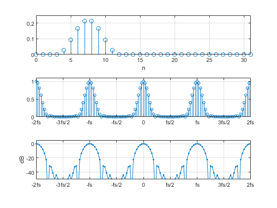
Figure 1. Periodic Spectrum of a sampled time signal.
Top: sampled time signal Middle: Spectrum magnitude Bottom: Spectrum dB-magnitude
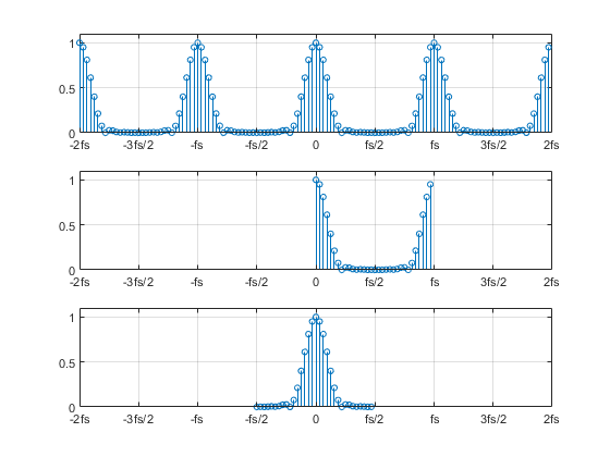
Figure 2. DFT magnitude |X(k)| for different frequency ranges.
Top: k = -2N to 2N-1 results in f = -2fs to fs(2N-1)/N
Middle: Conventional DFT. k = 0 to N-1 results in f = 0 to fs(N-1)/N
Bottom: DFT centered at f = 0. k= -N/2 to N/2-1 results in f = -fs/2 to fs(N/2-1)/N
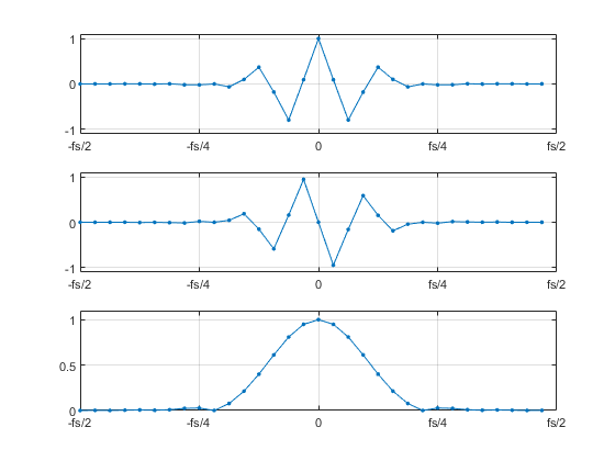
Figure 3. DFT evaluated over k = -N/2 to N/2-1 or f = -fs/2 to fs(N/2-1)/N
Top: Real part, showing even symmetry.
Middle: Imaginary part, showing odd symmetry.
Bottom: Magnitude.
Appendix Matlab Code to Evaluate DFT over several periods of its spectrum
For this example, the time signal is a Hann, or Hanning, pulse [4, 5] with the formula
x(n) = K*(1 – cos(2πn/P)),
where P = 9 and n= 0: P. This pulse is then padded with leading and following zeros to length N= 32.
% extended_dft.m   3/4/19 Neil Robertson
% compute dft using its definition
% k = -2*N:2*N-1f = -2fs:2fs
%
fs= 100;                    % Hz sample frequency (arbitrary value)
N= 32;                      % number of time samples
% sampled time signal of length N
x= [0 0 0 0  7 24 43 55  55 43 24 7  0 0 0 0  0 0 0 0  0 0 0 0 ...
    0 0 0 0  0 0 0 0]/258;
% Compute DFT
M= 4*N;                         % number of frequency samples
for k= -M/2:M/2-1               % frequency index
    f(k+ M/2+ 1)= k*fs/N;       % frequency vector. index range is 1:M
    sum_n= 0;
    for n= 0:N-1                % time index
        sum_n= sum_n + x(n+1)*exp(-j*2*pi*k*n/N);    % DFT sum for X(k)
    end
    X(k+ M/2+ 1)= sum_n;         % DFT vector.  index range is 1:M
end
Xreal= real(X);
Ximag= imag(X);
Xmag= sqrt(Xreal.^2 + Ximag.^2);         % DFT magnitude vector
XdB= 20*log10(Xmag);                     % DFT dB-magnitude vector
%
%
%
% plot x, Xmag, and XdB
subplot(311),stem(0:N-1,x),grid
axis([0 N-1 0 .25]),xlabel('n')
subplot(312),stem(f,Xmag,'markersize',4),grid
axis([-2*fs 2*fs 0 1.1])
xticks([-2*fs -3*fs/2 -fs -fs/2 0 fs/2 fs 3*fs/2 2*fs])
xticklabels({'-2fs','-3fs/2','-fs','-fs/2','0','fs/2','fs','3fs/2','2fs'})
subplot(313),plot(f,XdB,'.-','markersize',7),grid
axis([-2*fs 2*fs -50 5])
xticks([-2*fs -3*fs/2 -fs -fs/2 0 fs/2 fs 3*fs/2 2*fs])
xticklabels({'-2fs','-3fs/2','-fs','-fs/2','0','fs/2','fs','3fs/2','2fs'})
ylabel('dB')
References
- Oppenheim, Alan V. and Shafer, Ronald W., Discrete-Time Signal Processing, Prentice Hall, 1989, section 3.2.
- Rice, Michael, Digital Communications, a Discrete-Time Approach, Pearson Prentice Hall, 2009, section 2.6.1.
- Lyons, Richard G. , Understanding Digital Signal Processing, 2nd Ed., Prentice Hall, 2004, Chapter 4.
- Mathworks website, https://www.mathworks.com/help/signal/ref/hann.html
- Oppenheim and Shafer, Op. Cit., p. 447.
March 2019 Neil Robertson
- Comments
- Write a Comment Select to add a comment

Hi Neil,
That is neat and useful. By the way I happened to compare DFT equation Vs iDFT. Apart from scaling,they look exactly same except for j/-j operator. Or am I wrong? So I tried both equations on a single tone @ + 0.1 Fs and can see DFT gives single line @ +0.1Fs as expected while iDFT gives same but @ -0.1Fs.
I wonder if the sign of (j) operator is actually chosen on arbitrary basis between DFT and iDFT. Moreover, I find it a bit hard to imagine how come one way the equation converts to frequency domain while the other way it converts to time domain.
Thanks
Kaz

Hi Kaz,
I'm glad you liked the article.
The continuous fourier transform is the integral of f(t)exp(-jwt)dt.
The inverse is the integral of 1/(2pi) * F(w)exp(jwt)dt.
If I ever knew how this arises, I have forgotten. Here is an article on computing the IDFT, by Rick Lyons:
Thanks Neil,
swapping Re/Im at input/output to fft, or inverting (Im) in effect forces +f of input to -f then back to +f at output... and this agrees with my test above. In practice we do rewiring of Re/Im as it costs nothing. Other three methods are costly but interesting.
Thus it confirms my conclusion that DFT and iDFT are almost same apart from transpose of Re/im input/outputs or cos/sin terms.
I can imagine DFT correlates set of cos/sin and picks up maximum as new samples indexed from zero to N-1. Hence it measures frequency content.
iDFT does same but using transposed cos/sin. How come this means un-corelating and converting from frequency domain to time domain. I can't "imagine".
Regards
Kaz

Hi kaz.
Both the DFT and the iDFT perform correlations.
Hi Rick,
Thanks, yes the equations are very much same concept but this by itself raises the question.
Imagine a single tone, do fft and we get a single line.
if we now think of fft as conversion from time domain to frequency domain then all makes sense as we are correlating with a set of bin frequencies and end up with single line as expected. No problem in concept.
If we do ifft on this single line we expect single tone and we get it.
However for ifft we are correlating same way as if we entered a single line to fft.
The ifft equations should conceptually convert from frequency domain back to time domain but it uses same equation that we used to move from time domain to frequency domain. so we are still trying to find out how much is there from each bin frequencies as if we are not in frequency domain but convert from time domain to frequency domain.
I can see that mathematically ifft inverts the fft but I believe as such the concept of time domain versus frequency domain is just a convenient byproduct.
Kaz

The choice of sign for which is forward and which is backward is by convention. So is the normalization factor.
The reason that the convention of using a negative sign is a little preferable is how the arg of the bin value relates to the phase of the signal. This is clearest in the complex case:
$$ x[n] = e^{ \omega n + \phi } $$
Suppose the DFT frame is a whole number of cycles, and $ k = \omega \cdot \frac{N}{2\pi} $, then
$$ X[k] = (value) \cdot e^{\phi} $$
By using the negative sign in the forward DFT the signs on $\phi$ align, that make sense.
What I have an issue with is the normalization factor convention. I can understand a factor of "1" in library routines to save a multiply, but when you are doing the math, it is less sensible.
The "true" normalization factor should be $ \frac{1}{\sqrt{N}} $, but that is a pain to deal with in practicality. It is the "true" one because it applies to the forward and inverse DFT making the operations "multiplications of unitary matrices" in Linear Algebra terminology. The common convention of using "1" for the forward and "1/N" for the inverse is backward in my opinion. It should be the reverse.
If you use the reverse, as I advocate, then the $(value)$ in the above equation becomes "1" for complex signals and "1/2" for real ones, making the interpretation of bin values independent of the sample count. This is much more sensible and why I stubbornly use a "1/N" in all my articles even though it is immaterial for frequency calculations since those are amplitude independent.
In addition, in the cases when your DFT frame covering a whole number of cycles of a periodic signal, then the coefficients for the Fourier Series for the continuous function can be read straight from the DFT bin values. This should be the clincher.
Ced
Thanks Ced,
For FPGA/ASIC platforms as opposed to math or soft platforms we got commercial fft/ifft cores that scale by sqrt(N) for either direction. Still not practical due to bit growth limitation. I normally scale output back by 1/sqrt(N) using precomputed single constant plus one multiplier.
I am still not sure how to mentally explain the ifft equation...
Kaz
Conceptually (and literally), the bin values are the coefficients to the Sine and Cosine functions that reconstruct your function.
The inverse DFT is that reconstruction.
Hi Neil.
Your interesting blog brings up a philosophical question that deserves contemplation. That is, "Is it possible for a discrete sampled sine wave to have a frequency more positive than Fs/2 Hz?"
Rick,
I assume you mean a real sine wave. Let its frequency = f0. According to all the textbooks, it has an infinite number of frequency pairs at +/-f0, fs+/-f0, 2*fs+/-f0...
You could approach this in the real world by sampling a sine wave with a pulse train having very narrow pulses. The amplitude of the resulting spectral lines would roll off slowly vs f, and the amplitude would be proportional to the energy in the pulse. If the pulse width were, say, 1 ns, it would be good to have a large pulse amplitude (100 volts?)
Then you could put a bpf centered at the frequency of one of the spectral lines and you should get a sine out.
Neil
One detail: when I refer to sampling the sinewave with a pulse train with narrow pulses, this could either be a switch or a multiplier. If it is a multiplier, the amplitude of the pulse train obviously affects the output amplitude.
The final filtered amplitude would then depend on the pulse width and pulse amplitude.
Neil
when converted through DAC you can exploit the faster copies at multiples of that provided you filter accordingly.
Kaz
I guess the philosophical part is when you decide that the ADC output samples are impulses. This is what makes the math work.
Then, when you get to the DAC, you have to convert the perfect impulses into something else -- typically square pulses, which cause the higher frequency copies to follow the sinx/x curve.
Neil
@ Neil.
Hi. For me the philosophical question is: "Is it possible to generate a discrete sampled sine wave (a sequence of numbers) whose frequency is more positive than +Fs/2 Hz?"
And while you at it, can you tell me how many angels can fit on the head of a pin?
@ kaz.
Hi. Your 1st sentence implies to me that you believe that no discrete sine wave can have a frequency more positive than +Fs/2 Hz. Am I correct?
Hi Rick,
Yes the discrete domain cannot have frequencies outside Nyquist rule.
Any frequency outside this range cannot exist in discrete domain.
However I noticed some programmers computationally enter high frequencies in the generation equation that will appear as alias within the legal range.
If we sample high frequency signal from real world at ADC it will alias into legal domain.
If we want DAC to produce higher frequencies outside the legal range then yes you can exploit copies at DAC output.
I am sure you know that but curious what is in your mind.
Kaz
@Neil.
Hi. This signal you refer to that can be applied to a bandpass filter, is that signal an analog signal or a discrete sequence of numerical samples (a discrete signal)?
Rick,
My signal was an analog signal that is the product of a sinewave and a pulse train. So it does not fit your description of a discrete signal.
Any analog sinewave above fs/2 will produce an alias below fs/2 when discretized. I guess we can believe in the higher frequency images or not, as we prefer.
Neil
hi I have a quastion, i dont underestand why do we consider the amount of k,(k=N/2) ?what is the problem whitH k=N?
Hi Saraktb,
There is no problem with letting k go from 0 to N-1. However, since the spectrum of a real signal is symmetrical, all the information is contained in the range k = 0 to N/2-1. The range of k= N/2 to N-1 is just an image.
Note the matlab fft function returns all N points of the DFT, so you can choose to keep all N points or just look at N/2 points.
regards,
Neil
To post reply to a comment, click on the 'reply' button attached to each comment. To post a new comment (not a reply to a comment) check out the 'Write a Comment' tab at the top of the comments.
Please login (on the right) if you already have an account on this platform.
Otherwise, please use this form to register (free) an join one of the largest online community for Electrical/Embedded/DSP/FPGA/ML engineers:


