Compute Images/Aliases of CIC Interpolators/Decimators

• Matlab
• Basics
• Multirate DSP

Cascade-Integrator-Comb (CIC) filters are efficient fixed-point interpolators or decimators.  For these filters, all coefficients are equal to 1, and there are no multipliers.  They are typically used when a large change in sample rate is needed.  This article provides two very simple Matlab functions that can be used to compute the spectral images of CIC interpolators and the aliases of CIC decimators.

1.  CIC Interpolators

Figure 1 shows three interpolate-by-M filters (M is an integer) that all have the same impulse response [1,2].  Figure 1a performs upsampling by M, followed by two M-tap boxcar filters.  Figure 1b replaces each boxcar filter with an equivalent implementation consisting of a comb and integrator.  The comb sections each have a delay of M samples.  Finally, Figure 1c groups combs together and integrators together, with the upsampling function between them.  The combs now operate at the lower input sample rate, and the comb delay is one sample instead of M samples.  This Hogenauer filter [3] is the most efficient way to implement a CIC filter.

The frequency response of a single stage boxcar or CIC interpolator is:

$$H(f)=\frac{sin(\pi fMT_s)}{sin(\pi fT_s)} \qquad(1)$$

where T_s is the interpolator’s output sample time.  For an N-stage filter, the frequency response is:

$$H(f)=\left[\frac{sin(\pi fMT_s)}{sin(\pi fT_s)}\right]^N \qquad(2)$$

The magnitude response has nulls at multiples of the input sample rate.

Equation 1 is called the Dirichlet, or aliased sinc, function.  One shouldn’t confuse it with the spectrum of a continuous time pulse of length T, which is $X(f)=sin(\pi fT)/(\pi fT)$.  X(f) lacks the sine in the denominator.

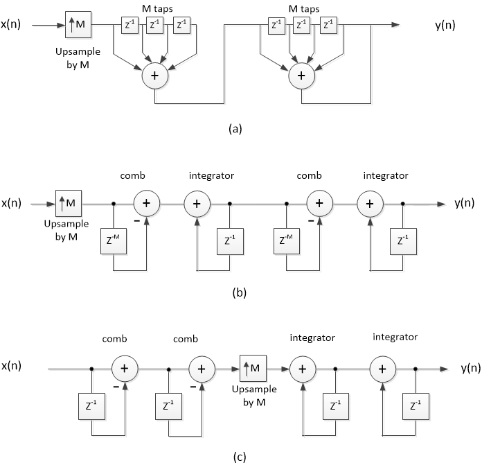
Figure 1.  Equivalent two-stage interpolate-by-M filters.

a) Cascaded boxcars    b) CIC    c) Hogenauer CIC

Since Figure 1a has the same impulse response as the CIC interpolators, we can use it to model them.  We’ll compute an N-stage impulse response simply by performing repeated convolutions of the boxcar impulse response.  A Matlab function boxcar_interp.m is listed in Appendix A of the PDF version.  Note that the boxcar coefficients are scaled by 1/M in the function.

Here is an example to compute the impulse response and magnitude response of an M= 40 CIC filter with 4 stages:

    M= 40;                   % interpolation ratio
    Nstages= 4;              % number of CIC stages
    x= [1 0 0 0];            % impulse input
    y= boxcar_interp(x,M,Nstages);    % perform interpolation

The impulse response y is plotted in Figure 2 (top).  Given an input sample rate of 100 Hz and output sample rate of M*f_{s_in} = 40*100 = 4000 Hz, the magnitude response can be calculated as follows:

    fs_in= 100;                            % Hz input sample rate
    [h,f]= freqz(y/M,1,1024,M*fs_in);      % /M compensates for upsampler gain
    H= 20*log10(abs(h));                   % dB magnitude response

The magnitude response is plotted in Figure 2 (bottom).  The response has nulls at multiples of f_{s_in} = 100 Hz.

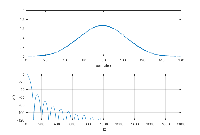
Figure 2.  Top:  Impulse response of 4-stage CIC Interpolator, M= 40.

Bottom:  Magnitude response for input sample rate = 100 Hz.

Now let’s look at the impulse response and magnitude response of a CIC interpolator versus the number of stages.  The example is clearer if we keep M fairly low, so we’ll use M = 8.  Here is the code for a single stage CIC interpolator with M = 8:

    fs= 1;                           % Hz output sample rate
    M= 8;                            % interpolation ratio
    x= [1 0 0 0];                    % impulse input signal
    y1= boxcar_interp(x,M,1);        % find one-stage interpolator output
    [h,f]= freqz(y1/M,1,2048,fs);    % /M compensates for upsampler gain
    H1= 20*log10(abs(h));            % dB magnitude response

The impulse response shown in Figure 3a is that of a boxcar filter.  The dB-magnitude response is shown as the top curve in Figure 4, which agrees with Equation 1.  We can repeat the above for a two-stage interpolator, where everything is the same except for the function call and output signal name.  The function call is:

    y2= boxcar_interp(x,M,2);        % find 2-stage interpolator output

The function convolves two boxcar responses to obtain the triangular impulse response shown in Figure 3b.  Similarly, convolving the triangle response with a boxcar gives the impulse response of a three-stage filter shown in Figures 3c, and one more convolution yields the four-stage impulse response of Figure 3d.  The magnitude responses (calculated by freqz or by Equation 2) of all filters are plotted in Figure 4.  As shown, the stopband lobe levels decrease with increasing number of stages, while the bandwidths of the stopbands centered at multiples of the input sample rate (f_s/M) increase.  Note, however, that the 3-dB passband bandwidth decreases vs. number of stages.

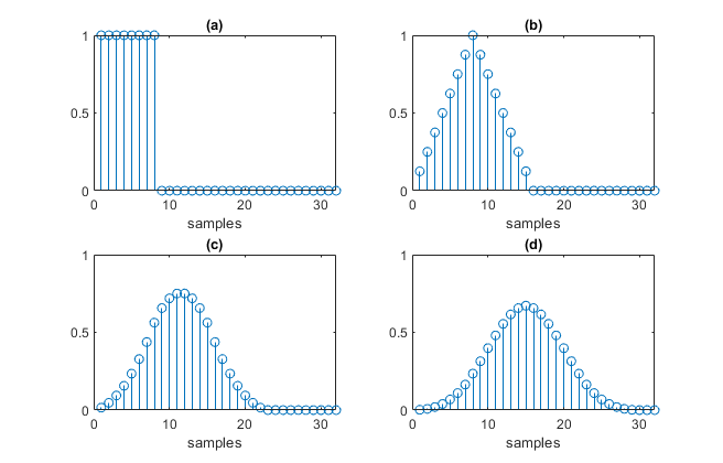
Figure 3.  Impulse responses of CIC interpolators with M = 8.

a) One-stage    b) Two-stage    c) Three-stage    d) Four-stage.

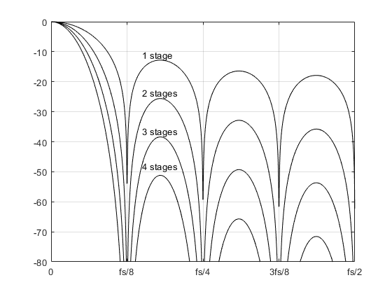
Figure 4.  Magnitude responses of CIC filters with M = 8.  f_s = output sample rate.

2.  Interpolator Output Spectrum with Images

Given an input time sequence, it’s easy to compute the interpolator’s output signal and spectrum, including images.  Here’s an example that computes the output of a three-stage, M = 8 interpolator having multiple sine inputs sampled at 100 Hz.  The following code generates the sines, performs the interpolation, and computes the spectrum of the output signal.  The function psd_simple.m, which I described in a post [4], is listed in Appendix B of the PDF version.

    M= 8;                        % interpolation ratio
    Nstages= 3;                  % number of stages
    % compute multiple-sine input x
    fs_in= 100;                  % Hz input sample rate
    T= 1/fs_in;                  % s input sample time
    f0= 5; f1= 9; f2= 13;        % Hz sine frequencies
    N= 256;
    n= 0:N-1;                    % time index
    A= sqrt(2);                  % amplitude of each sinewave
    x= A*sin(2*pi*f0*n*T) + A*sin(2*pi*f1*n*T) + A*sin(2*pi*f2*n*T);
    %
    y= boxcar_interp(x,M,Nstages);         % perform interpolation
    [PdB,f]= psd_simple(y,M*N,M*fs_in);    % output spectrum

The spectrum of the interpolator output y (f_s = 800 Hz) is plotted in Figure 5, along with the interpolator magnitude response (dashed line).  The spectrum shows images centered at multiples of f_{s_in} = 100 Hz.  The large images at 87, 113, 187, 213, … Hz are due to the sine input at 13 Hz.

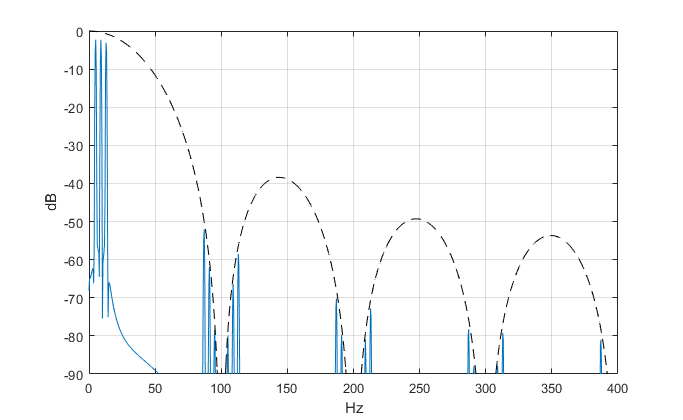
Figure 5.  Three-stage CIC interpolator output spectrum.   M= 8, input sample rate = 100 Hz.

3.  CIC Decimators

Figure 6 shows equivalent implementations of two-stage decimate-by-M filters [1,2].  Figures 6a and 6b are like the interpolators in Figures 1a and 1b, except the upsampler at the input has been replaced by a downsampler at the output.  Figure 6c groups the integrators on the input side and the combs on the lower-rate output side, with a downsampler between them.  The comb delay is one sample instead of M samples.  The integrators must be implemented using two’s-complement arithmetic such that they roll over when the signal amplitude exceeds the number of bits in the adder [1,2,3].

For a given value of M and a given number of stages, a decimator has the same frequency response as an interpolator, when evaluated relative to the decimator's input sample rate.  This is apparent from comparing Figure 1a for an interpolator to Figure 6a for a decimator.

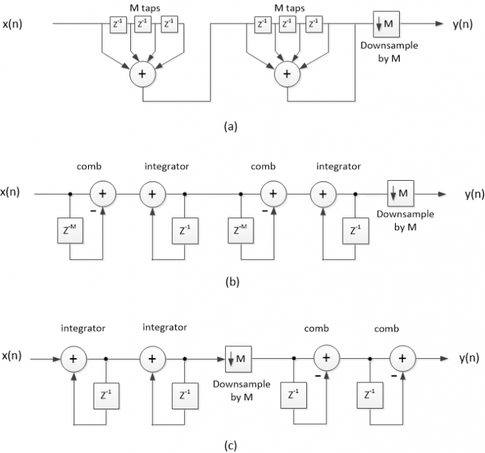
Figure 6.  Equivalent two-stage decimate-by-M filters.

a) Cascaded boxcars    b) CIC    c) Hogenauer CIC

4.  Decimator Output Spectrum with Aliases

To find the time response of a CIC decimator, we’ll use the equivalent cascaded-boxcar decimator of Figure 6a.  The N-stage impulse response (before downsampling) is computed by performing repeated convolutions of the boxcar impulse response.  The function boxcar_dec.m is listed in Appendix A of the PDF version.

Here’s an example using the same parameters -- M = 8 and Nstages = 3 -- used in section 2 for an interpolator.  The input signal consists of four unwanted sines at different frequencies, sampled at 800 Hz.  The following code generates the sines, performs decimation, and computes the spectra of the input and output signals.  The function psd_simple.m is listed in Appendix B of the PDF version.

    M= 8;                      % decimation ratio
    Nstages= 3;                % number of stages
    fs_in= 800;                % Hz input sample rate
    % multiple-sine input to decimator
    T= 1/fs_in;                % s input sample time
    f1= 90; f2= 94; f3= 214; f4= 218;    % sine frequencies
    N= 4096;
    n= 0:N-1;                  % time index
    A= sqrt(2);                % amplitude of each sinewave
    x= A*sin(2*pi*f1*n*T) + A*sin(2*pi*f2*n*T) + ...
       A*sin(2*pi*f3*n*T) +A*sin(2*pi*f4*n*T);
    %    
    [PdB_in,fin]= psd_simple(x,N,fs_in);          % input spectrum
    y= boxcar_dec(x,M,Nstages);                   % perform decimation
    [PdB_out,fout]= psd_simple(y,N/M,fs_in/M);    % output spectrum

The input spectrum is shown in the top of Figure 7, along with the decimator’s magnitude response (dashed line), which is the same as that of the interpolator in section 2.  To avoid hiding the aliases, there is no “desired” input signal, just four unwanted sinewaves.  Output sample rate is 100 Hz, and the output spectrum is shown in the bottom of Figure 7.  The output spectrum shows the aliases:

6 Hz due to input at 94 Hz; 10 Hz due to input at 90 Hz;

14 Hz due to input at 214 Hz; 18 Hz due to input at 218 Hz.

Note that the decimator output y has 515 samples, enough to provide adequate resolution in the spectrum.  To get the 515 samples, we needed the input x to have 4096 samples (roughly M times the length of y).

The function boxcar_dec.m can also be used to compute aliases due to modulated input signals; an example using the same decimator as above is shown in Figure 8.  Again, to avoid hiding the aliases, there is no desired input signal, just the unwanted signals.

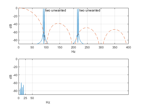
Figure 7.  Three-stage CIC decimator example.  M= 8, input sample rate = 800 Hz.

top: Input signal spectrum.    bottom: Output spectrum.

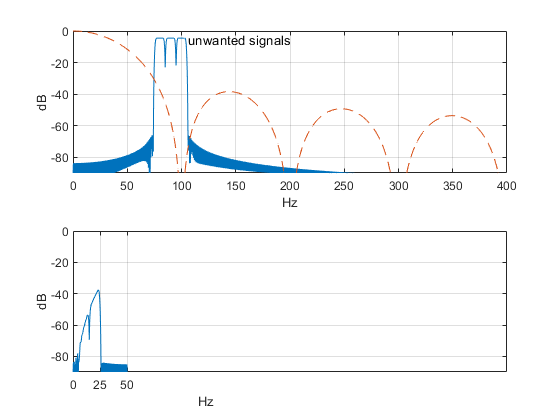
Figure 8.  Another three-stage CIC decimator example.  M= 8, input sample rate = 800 Hz.

top: Input signal spectrum.    bottom: output spectrum.

See PDF version for Appendix A and Appendix B.

References

1.  Harris, Fredric J., Multirate Signal Processing for Communication Systems, Prentice Hall, 2004, Ch. 11.

2.  Lyons, Richard G., Understanding Digital Signal Processing, Third Ed., Prentice Hall, 2011, section 10.14

3.  Hogenauer, Eugene B., “An Economical Class of Digital Filters for Decimation and Interpolation”, IEEE Trans. On Acoustics, Speech, and Signal Processing, vol. ASSP-29, No. 2, April 1981, pp. 155 – 162.

4.  Robertson, Neil C., “A Simplified Matlab Function for Power Spectral Density”, DSPrelated.com, March, 2020, https://www.dsprelated.com/showarticle/1333.php

Neil Robertson           November, 2020

Sign in