Setting Carrier to Noise Ratio in Simulations

• Matlab
• Tutorials

When simulating digital receivers, we often want to check performance with added Gaussian noise.  In this article, I’ll derive the simple equations for the rms noise level needed to produce a desired carrier to noise ratio (CNR or C/N).  I also provide a short Matlab function to generate a noise vector of the desired level for a given signal vector.

Definition of C/N

The Carrier to noise ratio is defined as the ratio of average signal power to noise power for a modulated signal.  There isn’t normally an unmodulated carrier available to measure, so we just measure the signal’s average power. This average signal power is the “C” in C/N.  It is acceptable to measure the signal power with noise present, as long as C/N is greater than 10 dB or so.  The noise power is the average power of the noise measured over a defined bandwidth in the absence of the signal.  The bandwidth used to measure the noise power is called the noise equivalent bandwidth of the receiver.

In this article, I’ll use the following steps to set the C/N:

• Compute the noise density N₀ using the noise equivalent bandwidth.
• Use N₀ to compute the rms level of the noise.
• Generate a noise vector using the Matlab function randn [1,2]. 

Computing noise density N₀ using noise equivalent bandwidth

Figure 1 shows a system where Gaussian noise is added to the transmitted signal to obtain a given C/N at the receiver.  The receiver includes a bandpass channel filter before the demodulator.  This represents any of the various types of receive filter that could be used, such as an intermediate frequency (IF) filter or the baseband I/Q filters of a quadrature demodulator.  The filter’s purpose is to attenuate out of band noise and interference.  The C/N is defined at the output of the filter.

Our goal is to find the noise density N₀ (W/Hz) that results in the desired C/N.  We will assume the transmitter’s noise contribution can be neglected.  Figure 2 shows the filter response, which we assume has a passband gain of 1.0.  We further assume that the filter causes negligible attenuation of the signal power.  The figure also shows the response of an ideal bandpass filter that has the same output power for input noise power density N₀.  The bandwidth of the ideal filter is called the noise-equivalent bandwidth B_eq [3].

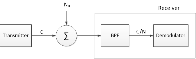
Figure 1.  Adding Gaussian noise (N₀ W/Hz) to a transmitted signal to achieve a given C/N.

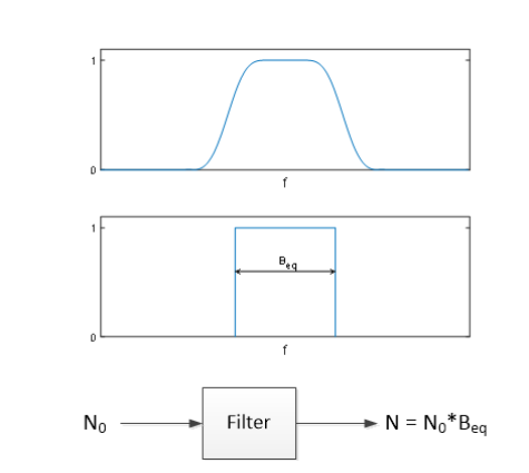
Figure 2.  Bandpass filter magnitude response and response of equivalent ideal filter.

                Output noise power N = N₀*B_eq.

Once we know B_eq for our filter, then we can compute the output noise power as:

$$N= N_0 B_{eq} \qquad (1) $$

(make note that N is noise power and not number of samples!)  If we know B_eq, we can then solve Eq. (1) for N₀.  For a discrete-time system,

$$N= N_b B_{eqb} \qquad (2) $$

Where N_b is in W/bin and B_eqb is in bins.  We can find B_eqb as follows for a discrete-time filter H(k).  The noise power density at the output of H(k) is:

$$ noise\ power\ density = N_b|H(k)|^2 \qquad W/bin $$

The average noise power is the sum of the noise power density over k:

$$ N= N_b \sum_{k=0}^{M/2-1}|H(k)|^2 \quad W \qquad (3) $$

where M/2 is the number of bins in the one-sided frequency response H(k).

Equating (2) and (3), we get:

$$ B_{eqb}= \sum_{k=0}^{M/2-1}|H(k)|^2 \quad bins \qquad (4) $$

Given sample frequency of f_s, there are f_s/M Hz per bin, and the noise equivalent bandwidth in Hz is:

$$ B_{eq}= \frac{f_s}{M}\sum_{k=0}^{M/2-1}|H(k)|^2 \quad Hz \qquad (5) $$

It turns out that B_eq can usually be computed directly from the discrete-time filter’s coefficients or impulse response:  the method is described in Appendix B.  Given C, C/N, and B_eq, we can now easily compute N₀ using the following two equations:

$$ N= \frac{1}{C/N}*C \qquad (6) $$

$$ N_0= \frac {N}{B_{eq}} \qquad (7) $$

Computing rms value of noise given N₀

Now that we know how to calculate N₀, we’ll use it to find the rms level (standard deviation) of the Gaussian noise.  Figure 3 shows the one-sided spectrum of discrete-time Gaussian noise with noise density of N₀ W/Hz.  We can write N₀ as simply:

$$ N_0= \frac{average\ noise\ power}{f_s/2} = \frac {\sigma^2}{f_s/2} \quad W/Hz $$

Where σ² is the average power (variance) of the Gaussian noise.  Thus, the standard deviation of the noise is just:

$$ \sigma= \sqrt{N_0 f_s/2} \qquad (8) $$

We can now use Equations 6, 7, and 8 to set the level of Gaussian noise that produces a desired C/N.  Appendix A lists the Matlab function set_cnr that generates a Gaussian noise vector, given the following inputs:  a signal vector, B_eq, f_s, and the desired C/N.  The signal may be real or complex.

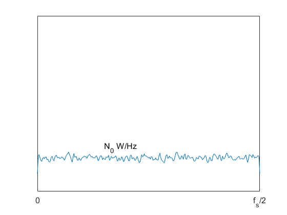
Figure 3.  Spectrum of Gaussian Noise (averaged)

Example 1.  Real QAM signal with square-root Nyquist filtering

For a real QAM signal, B_eq of the receiver’s root-Nyquist filter is equal to the symbol rate [4], which also happens to be the -3 dB bandwidth of the filter.  The following Matlab code generates a real QAM-16 signal, sets its C/N to 50 dB using set_cnr, and computes the resulting spectrum.  The Matlab functions qam_tx_real and psd_kaiser are listed in the PDF version, Appendices C and D, respectively. 

    Nsymbol= 4096;                 % Number of QAM symbols
    fs= 80;                        % Hz sample rate
    f0= 12.5;                      % Hz center frequency
    M= 16;                         % QAM order
    x= qam_tx_real(M,Nsymbol,f0,fs);    % QAM with 16 samples/symbol
    x= 4.5*x;                      % adjust signal level
    Beq= fs/16;                    % Hz noise bandwidth = fsymbol
    cnr_dB= 50;
    noise = set_cnr(x,Beq,cnr_dB,fs);    % noise vector
    y = x + noise;
    nfft= Nsymbol/4;
    [PdB1,f]= psd_kaiser(x,nfft,fs);    % averaged spectrum of x
    [PdB2,f]= psd_kaiser(y,nfft,fs);    % averaged spectrum of x + noise

Figure 4 shows the averaged spectrum of the QAM-16 signal before and after adding noise.  The signal is random, with a power density of P₀ W/Hz.  For our QAM system, we assume identical (matched) root-Nyquist filters in the transmitter and receiver. Total signal power out of the transmitter’s matched filter is then P₀*B_eq, while the noise power passed by the receiver’s matched filter is N₀*B_eq.  Thus:

C/N = P₀/N₀

Or, in terms of power per bin:

C/N = P_b/N_b

This means we can check the C/N as the dB-difference between P_b and N_b in the spectrum, as can be seen in Figure 4, where P_b ~= -10 dB and N_b ~= -60 dB. Finally, note that for accurate noise level, set_cnr requires that the C/N of the input signal x be much greater than cnr_dB.

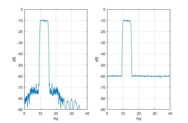
Figure 4.  Left:  Spectrum of QAM-16 signal x.   

Right:  Spectrum of y = x + noise for C/N = 50 dB.

Example 2.  Complex-baseband QAM signal with square-root Nyquist filtering

For a complex-baseband QAM receiver, Beq is the -3 dB bandwidth of the I and Q square-root Nyquist filters, which is equal to one-half the symbol rate.  The following Matlab code generates a complex-baseband QAM-16 signal and sets its C/N to 40 dB using set_cnr.  The Matlab function qam_tx_complex is listed in Appendix C of the PDF version. 

    Nsymbol= 4096;                % Number of QAM symbols
    fs= 80;                       % Hz sample rate
    M= 16;                        % QAM order
    [I,Q]= qam_tx_complex(M,Nsymbol);    % QAM with 4 samples/symbol
    x= 2*(I + j*Q);
    Beq= fs/8;                    % Hz noise bandwidth = fsymbol/2
    cnr_dB= 40;
    noise = set_cnr(x,Beq,cnr_dB,fs);    % noise vector
    y = x + noise;
    nfft= Nsymbol/4;
    [PdB1,f]= psd_kaiser(real(y),nfft,fs);    % averaged spectrum of I + noise
    [PdB2,f]= psd_kaiser(imag(y),nfft,fs);    % averaged spectrum of Q + noise
    [PdB3,f]= psd_kaiser(y,nfft,fs);       % averaged spectrum of I+j*Q + noise
    PdB3= fftshift(PdB3);

Figure 5 shows the spectra of I and Q with added noise.

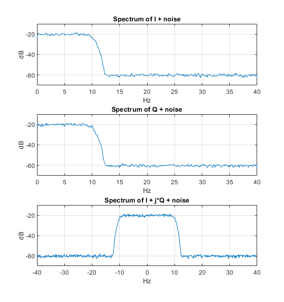
Figure 5.  Complex baseband QAM-16 signal with added noise, C/N = 40 dB.

Spectra of I, Q and I + jQ 

For Appendices, see the PDF version of this article.

References

1.  The Mathworks website, “randn” https://www.mathworks.com/help/matlab/ref/randn.html

2.  Moler, Cleve B., Numerical Computing with Matlab, siam, 2004, section 9.3

3.  Blinchikoff, Herman J. and Zverev, Anatol I., Filtering in the Time and Frequency Domains, Wiley, 1976, section 3.8.2.

4.  Cisco Systems, “Digital Transmission:Carrier-to-Noise Ratio, Signal-to-Noise Ratio, and Modulation Error Ratio”, 2006.

https://www.researchgate.net/profile/Dr_Asutosh_Kar/post/What_are_the_differences_between_signal_to_interference_ratio_and_Signal_to_noise_ratio2/attachment/59d637e4c49f478072ea510f/AS%3A273692343373824%401442264747403/download/Reference-1.pdf

5.  Mitra, Sanjit K., Digital Signal Processing (2^nd Ed.), McGraw-Hill, 2001, Table 3.5

6.  Frerking, Marvin E., Digital Signal Processing in Communication Systems, Chapman and Hall, 1994, p. 257.

7.  Robertson, Neil, “Third Order Distortion of a Digitally Modulated Signal”, DSPrelated.com, 2020,

https://www.dsprelated.com/showarticle/1355.php

8.  Robertson, Neil, “Model Signal Impairments at Complex Baseband”, DSPrelated.com, 2019,

https://www.dsprelated.com/showarticle/1312.php

9.  Robertson, Neil, “A Simplified Matlab Function for Power Spectral Density”, DSPrelated.com, 2020,

https://www.dsprelated.com/showarticle/1333.php

Neil Robertson               April, 2021

   revised 4/13/21

Sign in