Evaluate Noise Performance of Discrete-Time Differentiators

When it comes to noise, all differentiators are not created equal.  Figure 1 shows the magnitude response of two differentiators.  They both have a useful bandwidth of a little less than π/8 radians (based on maximum magnitude response error of 2%).  Suppose we apply a signal with Gaussian noise to each of these differentiators.  The sinusoidal signal with noise is shown in the top of Figure 2.  Signal frequency is π/12.5 radians.  The output of the so-called central-difference differentiator is shown in the middle plot, where we see that the signal has been attenuated more than the noise, resulting in obvious degradation.  The output of the “41 tap” differentiator is shown in the bottom plot.  Clearly, the noise performance of this latter differentiator is superior.

Referring back to Figure 1, it’s apparent the central-difference differentiator is passing much more noise energy at frequencies above π/8 radians than the 41 tap one.  The spectrum at the input of the differentiators is shown in Figure 3 (top).  The spectrum at the output of the central-difference differentiator is shown in Figure 3 (middle), where we see that the signal is attenuated about 12 dB, while the noise is barely reduced over much of the spectrum.  You could say the central-difference differentiator is an “open barn door” for noise.  The spectrum at the output of the “41 tap” differentiator is shown in Figure 3 (bottom):  the signal is also attenuated about 12 dB, but the noise power is much lower than that of the central-difference differentiator.

It would be nice to be able to quantify the difference in performance between differentiators.  In this article, I’ll introduce a Gaussian noise performance measure for differentiators that I’ll call Differentiator Noise Power Ratio.

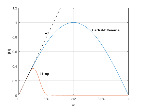
Figure 1.  Magnitude responses of a central-difference differentiator and a 41-tap

differentiator with equal usable bandwidth. 

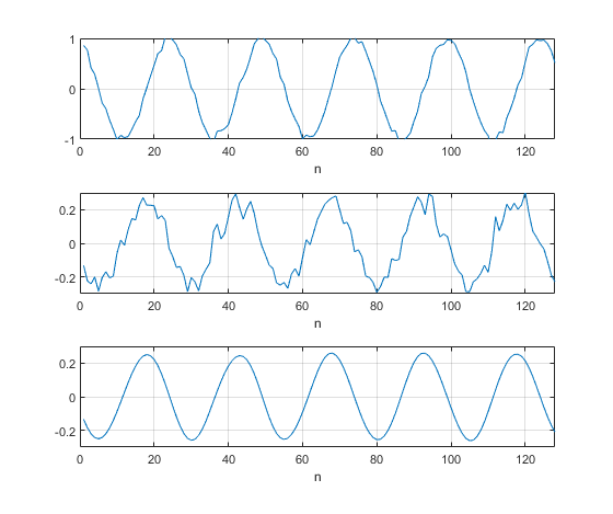
Figure 2.  Differentiator Noise Performance.

Top:  differentiator input signal with added Gaussian noise.

Middle:  output of central-difference differentiator (note change in vertical scale).

Bottom:  output of “41-tap” differentiator.

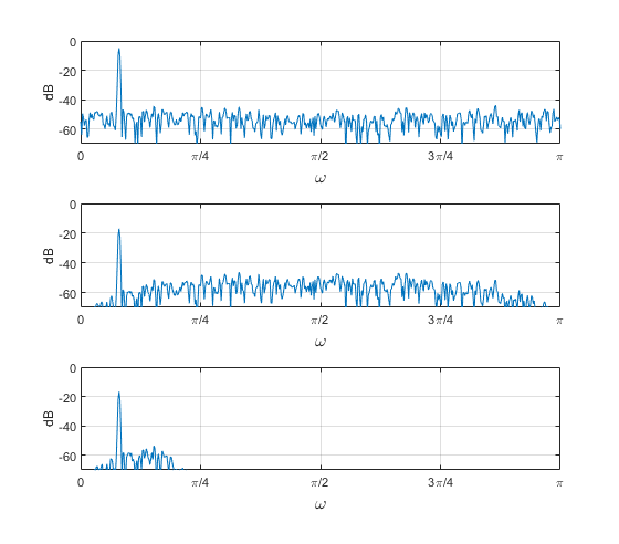
Figure 3.  Differentiator spectra.

Top:  input sinusoid with noise.   Middle:  Central-Difference output.   Bottom:  “41 tap” output.

Discrete-Time Differentiator Review

For continuous-time signals, the differentiation property of the Continuous Fourier Transform is:

$$\frac{d}{dt}x(t) \iff j\Omega X(\Omega) \qquad (1) $$

where Ω is continuous radian frequency.  There is no differentiation property of the Discrete Fourier Transform (DFT).  But given discrete signal x(n), it appears from Equation 1 that the DFT of its derivative should be jω X(ω), where ω= 2πf/f_s is discrete radian frequency, and f_s is the sample rate.

It turns out we can use a Finite Impulse Response (FIR) filter with real coefficients b(n) as an approximate differentiator:

$$ b(n) \circledast x(n) \iff H(\omega)X(\omega) \approx j\omega X(\omega) \qquad (2) $$

where $\circledast$ indicates discrete convolution, and the bi-directional arrow now represents the DFT.  The approximation sign means that the derivative is not exact.  What are the coefficients b(n)?  From Equation 2, we have:

$$ b(n) \iff H(\omega) \approx j\omega \qquad (3) $$

So, b(n) are coefficients whose DFT H(ω) is approximately jω.  Normally, the goal is that H(ω) approximate jω over some bandwidth less than 0 to π (0 to f_s/2).  Since jω is pure imaginary, we know from the symmetry properties of the DFT that b(n) must be odd-symmetric.  But odd-symmetric time functions are non-causal, so we typically only require odd symmetry with respect to the center of b(n).

A simple, often-used differentiator is the central-difference differentiator, who’s difference equation is:

$$ y(n)= 0.5x(n)-0.5x(n-2) \qquad (4) $$

The coefficients and block diagram are shown in Figure 4 a and b.  The z-domain transfer function is:

$$ H(z) = 0.5 - 0.5z^{-2} \qquad (5) $$

Letting z = e^jω, H(ω) is given by:

$$ H(\omega)=je^{-j\omega} sin(\omega) \qquad (6) $$

where the complex exponential term occurs because the center tap is delayed 1 sample from that of an odd-symmetric time function.  If need be, we can avoid this delay as follows.  The coefficients and block diagram of an odd-symmetric version of the differentiator are shown in Figures 4c and 4d.This filter has output y(n) time-aligned with the delayed input x(n-1).  The transfer function with respect to x(n-1) is:

$$ H(z) = 0.5z - 0.5z^{-1} \qquad (7) $$

resulting in

$$ H(\omega)= jsin(\omega) \qquad (8) $$

Note that the magnitude of H(ω) is the same for either differentiator:

$$ |H(\omega)| = |sin(\omega)| \qquad (9) $$

Recall that our goal is that H(ω) approximate jω, or at least that |H(ω)| approximate ω.  Equation 9 is plotted in Figure 1 as the central-difference response, along with |H| = ω (dashed line).  We see that the response approximates ω for small values of ω:

$$ |H(\omega)| \approx \omega,\; \omega<< \pi \quad (10) $$

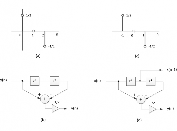
Figure 4.  Central-Difference Differentiator

a) Coefficients.   b) Block diagram.

c) Odd-symmetric Coefficients.   d) Odd-symmetric block diagram.

Differentiator Noise Power Ratio

Now we’ll develop our noise performance metric for differentiators.  As an example, we’ll use an FIR differentiator designed using the method described in [1].  I provide a Matlab function diff_synth.m for this purpose in Appendix A of the PDF version.  Suppose we want a differentiator with bandwidth approaching π/2 radians.  The desired magnitude response is shown in Figure 5 (top).  For number of taps = 25, diff_synth.m returns the coefficients shown in the bottom of Figure 5 (We’ll go into more detail about diff_synth.m later in this article).

The magnitude response of this filter is plotted in Figure 6 (top), along with the ideal response.  As you can see, the bandwidth of the filter is less than our original goal.  The response percent error is given by:

$$ \%\, error = 100 \frac{|H(k)|-\omega(k)}{\omega(k)} \qquad (11) $$

The percent error is plotted in Figure 6 (middle).  We can define the useful bandwidth of the filter based on some maximum allowed error.  For this example, if we choose maximum error of 2%, we get a bandwidth of ω_max ~= 0.39π as shown.

Figure 6 (bottom) plots |H(k)|, along with the response of an ideal differentiator with bandwidth ω_max.  The actual response obviously passes more noise power than the ideal response.  I define the quotient of Gaussian noise power passed by these two responses as the Differentiator Noise Power Ratio.

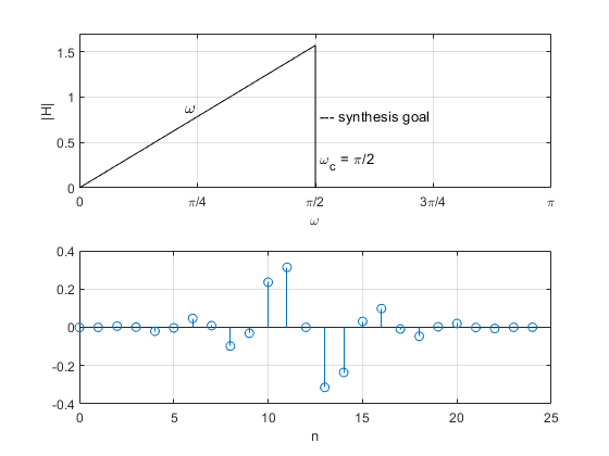
Figure 5.  Differentiator Example.   Top:  Desired response.

Bottom:  Coefficients of 25-tap differentiator.

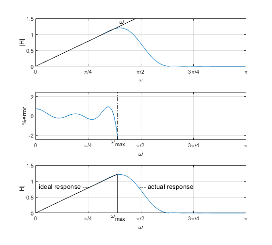
Figure 6.  Differentiator magnitude response and error.

Top:  Magnitude response and ideal response.

Middle:  Magnitude response error, showing frequency ω_max for 2% error.

Bottom:  Ideal response over 0 to ω_max and actual response.

Now we’ll develop a formula for Differentiator Noise Power Ratio.  Figure 7 shows a discrete-time differentiator with Gaussian noise input having a noise power density of N_b W/bin.

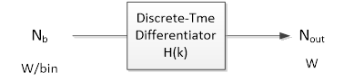
Figure 7.  Discrete-time differentiator with input noise density N_b W/bin.

At the output of the differentiator, we have:

$$ output\,noise\,power\,density= N_b|H(k)|^2 \quad W/bin \qquad (12) $$

where k = 0: M/2, and M/2 is the number of bins in the one-sided frequency response H(k).  The average output noise power is the sum of the noise power density over k:

$$ N_{out}= N_b\sum_{k=0}^{M/2-1}|H(k)|^2 \quad W \qquad (13) $$

We define the usable bandwidth of the differentiator as ω_max.  If we now consider the ideal differentiator with bandwidth ω_max (see Figure 6, bottom), the average output noise power is just:

$$ N_{out\,ideal}= N_b\sum_{k=0}^{k_{max}}\omega(k)^2 \quad W \qquad (14) $$

where k_max = Mω_max/(2π).  Taking the quotient of equations 13 and 14, we define the Differentiator Noise Power Ratio R as:

$$ R= \frac{N_{out}}{N_{out\,ideal}}= \frac{\sum_{k=0}^{M/2-1}|H(k)|^2} {\sum_{k=0}^{k_{max}}\omega(k)^2} \qquad (15) $$

For an ideal differentiator, R = 1.  In Appendix B of the PDF version, I derive a simpler expression for R based on ω_max and b(n):

$$ R = \frac{N_{out}}{N_{out\,ideal}} = \frac{3\pi}{\omega_{max}^3} \sum b(n)^2 \qquad (16) $$

We can state that The Signal to Noise Ratio (SNR) at the output of a given differentiator is reduced from that of an ideal differentiator of equal ω_max by a factor of R.  Equations 15 and 16 require that the passband slope of the differentiator magnitude response be 1.0.  It may sometimes be necessary to scale the coefficients b(n) to achieve this.  Keep in mind that the Differentiator Noise Power Ratio calculation is based on an assumption of Gaussian (white) noise.

What about the case of a differentiator cascaded with an FIR lowpass?  We can just convolve the coefficients of the differentiator with those of the lowpass, and use the resulting coefficients in Equation 16, making sure to include any change to ω_max.

Simple Differentiators

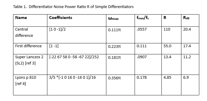
Table 1 lists Differentiator Noise Power Ratio R for several simple differentiators, where R was computed from Equation 16, and ω_max is based on 2% response error.  The magnitude responses of the differentiators are plotted in Figure 8.  Note that you don’t get to choose ω_max:  it is fixed for each differentiator. 

Using a different response error criterion would result in different values for R; for example, for a 5% error criterion, the central-difference differentiator would have ω_max = 0.175π and R = 28.3 (14.5 dB).  Also, for a narrowband signal, the differentiator response need only approximate linearity over a narrow frequency range.  In this case, the signal frequency could be yet higher, further improving noise performance. (Note that response slope would be less than 1, which could be compensated with a cascaded gain stage if desired).

Figure 9 plots R_dB vs f_max/f_s, where f_max/f_s = ω_max/(2π).  Given the existence of the ω_max³ term in the denominator of Equation 16, it is not surprising that performance improves with increasing f_max.  Keep in mind though, that if the signal spectrum occupies less than this full bandwidth, you will not obtain the calculated noise performance.  As shown, the central difference differentiator has the worst performance, although we should note that the first difference differentiator would perform poorly vs. high frequency noise or interference, given its high-pass magnitude response.

           Notes:

1.  ω_max = 2π f_max/f_s

2.  R_dB = 10*log₁₀(R)

3.  Maximum response error = 2%, except for Lyons, which has 2.5% error at low frequencies.

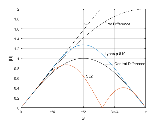
Figure 8.  Magnitude responses of simple differentiators.

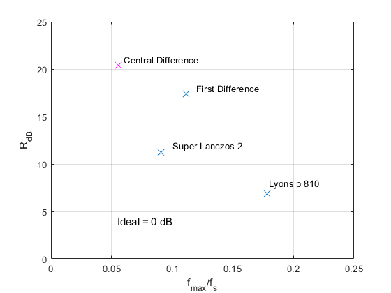
Figure 9.  Differentiator Noise Power Ratio R_dB vs. f_max/f_s for simple differentiators.

Maximum response error = 2%.

Custom Differentiators

The simple differentiators we discussed above are often appropriate, but they do not perform well in the presence of noise, and their usable bandwidth is arbitrary.  We can design better-performing differentiators using the following equation, which lets us choose a goal for ω_c [1]:

$$ b(k)= \frac{\omega_c cos(\omega_c k)}{\pi k} - \frac{sin(\omega_c k)}{\pi k^2} \qquad (17)  $$

where -N/2 <= k <= N/2 and N = ntaps – 1.  The Matlab function diff_synth.m listed in Appendix A of the PDF version uses this equation, along with a Hanning window function, to design custom differentiators.  Note that the differentiators’ usable bandwidth ω_max is less than ω_c.

As an example, suppose we want to design a 25-tap differentiator with ω_c = π/2, as shown in the top of Figure 5.  The Matlab code is:

    ntaps= 25;
    wc= pi/2;              % radians cutoff frequency goal
    b= diff_synth(ntaps,wc,2*pi);

The resulting coefficients are shown in Figure 5 (bottom).  The magnitude response and response percent error (Equation 11) are plotted in Figure 6.  They are computed as follows:

    [h,w]= freqz(b,1,256);
    H= abs(h);              % magnitude response
    e_pct= 100*(H-w)./w;    % percent error

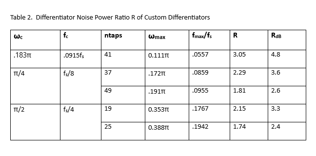
We can use diff_synth.m to design several custom differentiators with different lengths and different values of ω_max (or equivalently, f_max).  Table 2 lists parameters of five differentiators.  R_dB is plotted vs f_max/f_s for these differentiators in Figure 10.  Comparing Figure 10 to Figure 9, we see that the custom differentiators provide lower R_dB, at the expense of more taps.  Also, as you might expect, to obtain a given value of R_dB, fewer taps are required for differentiators with higher f_max/f_s vs. lower f_max/f_s.

Going back to our first example (Figures 1 - 3), we compared a central difference differentiator (R = 110, Table 1) and a custom “41 tap” differentiator (R = 3.05, Table 2), both having the same ω_max of 0.111π.  The difference in noise output power is 10*log₁₀(110/3.05) = 15.6 dB.  That is, the central-difference differentiator has 15.6 dB higher noise power output (15.6 dB worse SNR), given Gaussian noise at the input. 

Finally, another option for designing differentiators is the Matlab function firpm, with ‘ftype’ = ‘differentiator’.  This function uses the Parks-McClellan algorithm, and should be more efficient than the method used in diff_synth.m.

Notes:

1.  ω_max = 2π f_max/f_s

2.  R_dB = 10*log₁₀(R)

3.  Maximum response error = 2%

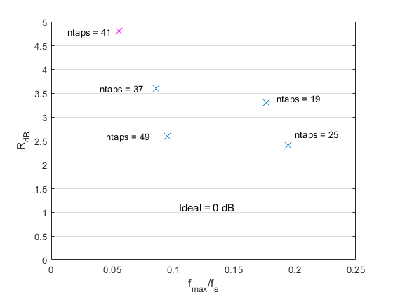
Figure 10.  Differentiator Noise Power Ratio R_dB vs. f_max/f_s for some custom

differentiators.  Maximum response error = 2%.

For Appendices, see the PDF version of this post.

References

1.  Lyons, Richard, Understanding Digital Signal Processing, 3^rd Ed., Prentice Hall, 2011, section 7.1.3.

2.  Lyons, section 7.1.2.

3.  Lyons, p 810.

4.  Mitra, Sanjit K., Digital Signal Processing, 2^nd Ed., McGraw-Hill, 2001, p 141.

5.  Spiegel, Murray R., et. al., Shaum’s Outlines Mathematical Handbook of Formulas and Tables, McGraw-Hill, 2018, equation 21.10.

                        Neil Robertson      March, 2022        Revised 3/29/22, 4/17/22, 12/5/22

Sign in