Decimators Using Cascaded Multiplierless Half-band Filters

• Matlab
• Multirate DSP

In my last post, I provided coefficients for several multiplierless half-band FIR filters [1].  In the comment section, Rick Lyons mentioned that such filters would be useful in a multi-stage decimator, as shown in Figure 1 for the decimate-by-8 case.  For such an arrangement, any subsequent multipliers save on resources, since they operate at 1/8^th of the maximum sample frequency or lower.  We’ll examine the frequency response and aliasing of a multiplierless decimate-by-8 cascade in this article, and we’ll also discuss an interpolator cascade using the same half-band filters.

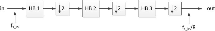
Figure 1.  Decimate-by-8 using half-band (HB) filters.

Half-band filters have passband and stopband frequency ranges that are symmetrical with respect to f_s/4, where f_s is sample rate.  Given a passband edge of f_pass, the stopband edge is:

$$ f_{stop}=\frac{f_s}{2} - f_{pass} \qquad(1) $$

An example half-band response is shown in Figure 2.  The result of the symmetry property is that, upon decimation by two, signals in the stopband are aliased into the passband, while signals between f_s/4 and the stopband are aliased above the passband.

For cascaded half-bands, suppose each filter has the same f_pass.  Then, from equation 1, f_stop must decrease after each stage.  We’ll illustrate this relationship in Example 1.

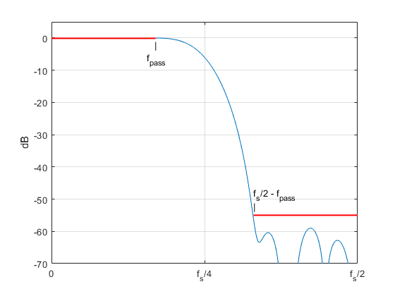
Figure 2.  23-tap half-band filter magnitude response, normalized for dc gain = 0 dB.

Example 1.  Decimate by 8

Figure 3 is a block diagram of a decimator-by-8 using three multiplierless half-band filters.  Input sample rate f_{s_in} is arbitrarily chosen as 1600 Hz, and output sample rate is 1600/8 = 200 Hz.  The filters have length 7, 11, and 23 taps, and their coefficients are:

b = [-1 0 9 16 9 0 -1]/32;                                   % fs = 1600 Hz

d = [8 0 -40 0 192 319 192 0 -40 0 8]/1024;     % fs = 800 Hz

g = [-2 0 7 0 -18 0 41 0 -92 0 320 512 ...

   320 0 -92 0 41 0 -18 0 7 0 -2]/1024;           % fs = 400 Hz

These filters were designed using the method described in an earlier post [2].  Implementation of the coefficients as sums of signed bit shifts is discussed at the end of this article.  The dc gain of the second filter is less than 1.0, so external gain K₂ = 25/16 is inserted after it to obtain approximately unity dc gain.

The stopband requirement is most difficult for the last filter, which has the lowest sample rate (400 Hz).  As can be seen from Figure 2, the 55 dB stopband edge of this 23-tap filter is about 0.33*f_s = 132 Hz.  Rearranging Equation 1, with f_s = 400 Hz, we get:

f_pass = f_s/2 – f_stop

f_pass = 400/2 – 132 = 68 Hz

For the most efficient design, the first two filters have the same passband of 68 Hz.  Again using Equation 1, we compute the required stopband edges:

First filter:  f_stop = 1600/2 – 68 = 732 Hz

Second filter:  f_stop = 800/2 – 68 = 332 Hz

So, the progression of stopband edges is 732/332/132 Hz.  Since the ratio of f_stop/f_pass decreases for each subsequent filter, the required minimum filter length increases.  The magnitude responses of the three filters are plotted in Figure 4, with the -55 dB stopbands shown in red.  The magnitude responses of the second and third half-bands have been extended up to f_{s_in}/2 (dashed lines).  As shown, the stopband edges of the first and second filters both meet the stopband frequency requirements.

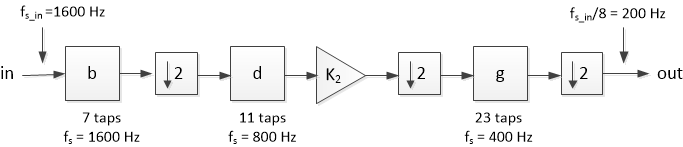
Figure 3.  Example decimate-by-8 using multiplierless half-band filters.

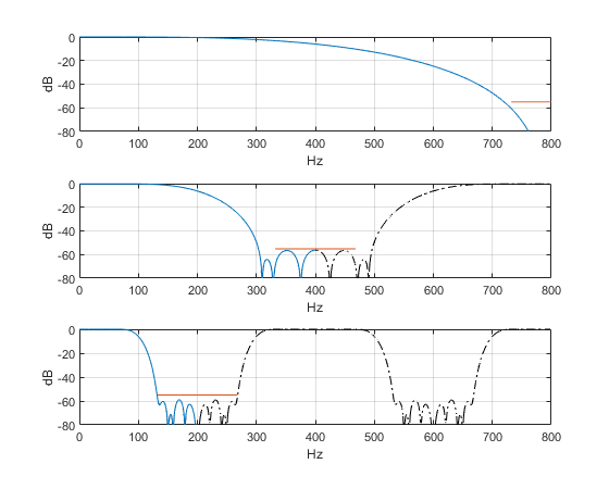
Figure 4.  Half-band filters for decimation by 8.  

Magnitude responses, stopband frequency range in red.

Top:  first HB, f_stop =732 Hz.   Middle:  second HB, f_stop =332 Hz.   Bottom:  third HB, f_stop = 132 Hz.

As I discussed in an earlier post [3], you can calculate the overall frequency response of a multistage decimator relative to the input sample rate.  For our case, this involves finding the impulse response of the equivalent single-stage decimate-by-8 filter.  The Matlab code to compute the impulse response and frequency response is as follows:

    fs_in= 1600;                % Hz input sample frequency
    fpass= 68;                  % Hz passband edge frequency
    K2= 25/16;                  % external gain for 2nd filter
    % half-band filter coefficients
    b= [-1 0 9 16 9 0 -1]/32;                  % fs = 1600 Hz
    d= K2*[8 0 -40 0 192 319 192 0 -40 0 8]/1024;    % fs = 800 Hz
    g= [-2 0 7 0 -18 0 41 0 -92 0 320 512 ...
       320 0 -92 0 41 0 -18 0 7 0 -2]/1024;      % fs = 400 Hz
    d_up= zeros(1,11*2);
    d_up(1:2:22)= d;               % upsample d by 4
    g_up= zeros(1,23*4);
    g_up(1:4:92)= g;               % upsample g by 8
    b23= conv(d_up,g_up);
    b123= conv(b,b23);             % overall impulse response at fs_in
    [H,f]= freqz(b123,1,512,fs_in);
    HdB= 20*log10(abs(H));         % dB overall magnitude response

The impulse response is plotted in the top of Figure 5, and the magnitude response is plotted in the bottom.  The stopbands shown fall at 200 Hz +/- f_pass, 400 Hz +/- f_pass, etc.  Why is the stopband attenuation so high near 600 Hz?  This is due to the attenuation of about 25 dB at 600 Hz of the first half-band filter (see Figure 4, top), which augments the stopband of the third half-band.   Additionally, the first half-band filter has 6 dB of attenuation at f_{s_in}/4 = 400 Hz.  The net result is that overall stopband attenuation of the decimator is greater than 60 dB, except near 132 Hz:  attenuation is 57 dB at 132 Hz.

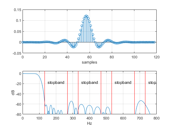
Figure 5.  Top:  Impulse response of equivalent single-stage decimate-by-8 filter.

Bottom:  Magnitude response is < -60 dB in stopbands, except near 132 Hz (-57 dB).

Now let’s try out the decimator with an input signal consisting of five sinewaves.  The following Matlab code generates the sinewaves, performs the decimation, and computes the spectrum of the output signal.

    % generate sinewaves
    N= 4096;             % number of samples
    n= 0:N-1;            % time index
    fref= 18;            % Hz freq of wanted signal
    f1= 120; f2= 292; f3= 352; f4= 740;    % Hz freqs of unwanted signals
    x= 1.9*(sin(2*pi*fref*n*Ts_in)+ sin(2*pi*f1*n*Ts_in)+ ...
    sin(2*pi*f2*n*Ts_in)+ sin(2*pi*f3*n*Ts_in)+ sin(2*pi*f4*n*Ts_in));
    %
    u= conv(x,b123);            % filter x using equivalent single-stage decimator
    y= u(1:8:end);              % downsample by 8
    [PdB,f]= psd_kaiser(y,512,fs_in/8);    % spectrum of decimator output</p>

The function psd_kaiser is listed in the appendix.  Note we could also have computed the output signal by applying the three decimation stages in order.

The input signal consists of one wanted sinewave at 18 Hz and four unwanted sinewaves at different frequencies.  Its spectrum is shown in the top of Figure 6, and the decimator magnitude response is shown in the bottom.  Note that the sinewaves at 352 and 740 Hz fall within stopbands, while the other two do not.

The decimator output spectrum is plotted in Figure 7.  The input frequency of each aliased component is shown in parenthesis on the plot.  The aliases of 352 and 740 Hz fall in the passband, and the other two aliases fall outside the passband.  These latter components can be attenuated by using a selective filter after the decimator.  Happily, the selective filter’s sample frequency is only 1/8^th of f_{s_in}.

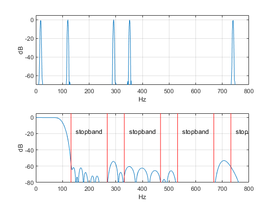
Figure 6.  Top:  Example input signal spectrum.   Bottom:  Decimator magnitude response.

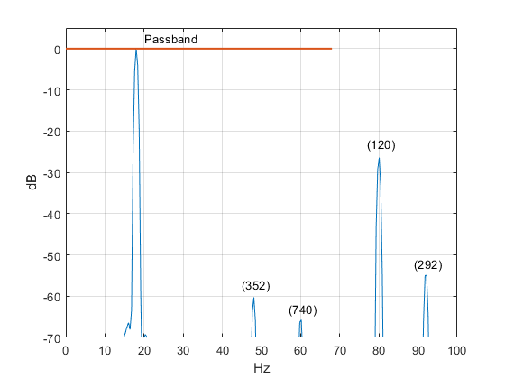
Figure 7.  Decimator output spectrum with aliases, f_s = 200 Hz.

Example 2.  Interpolate by 8

The same cascade of half-band filters in the reverse order can be used as an interpolator:  an interpolate-by-8 block diagram is shown in Figure 8.  Here, the 23-tap half-band with sample frequency of 400 Hz is the first filter in the chain, and the 7-tap half-band is the last.  Note that each upsample-by-2 function includes a gain of 2.  The passband edge frequency of 68 Hz is the same as the decimator’s.

The interpolator’s magnitude response, shown in the top of Figure 9, is identical to the decimator’s response of Figures 5 and 6.  The bottom of Figure 9 shows the interpolator’s output spectrum for input consisting of four sinewaves with frequencies of 10, 30, 50, and 68 Hz.  As shown, the interpolation images are centered at 200, 400, 600, and 800 Hz (the images centered at 600 Hz are less than -80 dB).

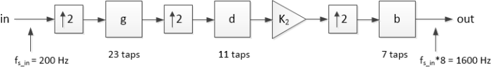
Figure 8.  Interpolator-by-8 using the same half-band filters as the decimator-by-8.

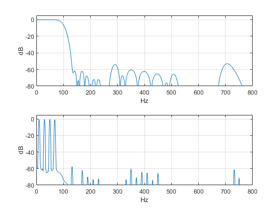
Figure 9.  Interpolation by 8.  Top:  Magnitude response of cascaded half-band filters.

Bottom:  Output spectrum for input of four sinewaves.

Multiplierless Implementation of Half-band Filters

I discussed multiplierless half-band filters in my last post [1].  There we found that the filter coefficients can be realized as signed bit-shifts (also called signed digits) or sums of signed bit-shifts.  Table 1 summarizes the coefficients and properties of the half-band filters.  All coefficients require three or fewer signed digits.  As an example, the block diagram of the 11-tap half-band is shown in Figure 10.  When used as a decimator or interpolator, this filter can be implemented as a polyphase design [4].  Here are the signed-digit implementations of the three filters used in this article:

7 tap:

b0 = b6 = -1/32

b2 = b4 = 9/32 = 1/4 + 1/32

b3 = 1/2

11 tap:

b0 = b10 = 1/128

b2 = b8 = -5/128 = -1/32 - 1/128

b4 = b6= 3/16     = 1/4 - 1/16  (or 1/8 + 1/16)

b5 = 319/1024     = 1/4 + 1/16 – 1/1024

23 tap:

b0 = b22 = -1/512

b2 = b20 = 7/1024  = 1/128 – 1/1024

b4 = b18 = -9/512   = -1/64 – 1/512

b6 = b16 = 41/1024 = 1/32 + 1/128 + 1/1024

b8 = b14 = -23/256  = -1/8 + 1/32 +1/256

b10 = b12 = 5/16     = 1/4 + 1/16

b11 = 1/2

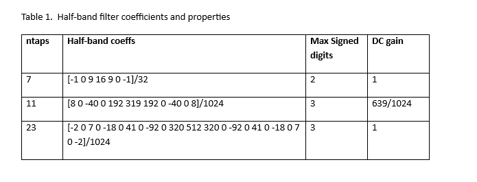
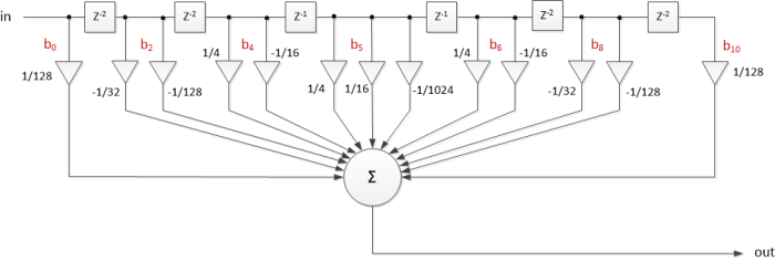
Figure 10.  11-tap half-band filter block diagram.  Blocks labeled z^-2 represent a delay of 2 samples.  For decimation or interpolation, the filter can be implemented as a polyphase design [4].

For the Appendix, see the PDF version.

References

1.  Robertson, Neil, “Multiplierless Half-band Filters and Hilbert Transformers”, DSPrelated.com, October, 2023,  https://www.dsprelated.com/showarticle/1585.php

2.  Robertson, Neil, “Matlab Code to Synthesize Multiplierless FIR Filters, DSPrelated.com, October, 2016, https://www.dsprelated.com/showarticle/1011.php

3.  Robertson, Neil, “Compute the Frequency Response of a Multistage Decimator”, DSPrelated.com, February, 2019, https://www.dsprelated.com/showarticle/1228.php

4.  Lyons, Richard G., Understanding Digital Signal Processing, 3rd Ed., Pearson, 2011, section 10.12.2

5.  Robertson, Neil, “A Simplified Matlab Function for Power Spectral Density”, DSPrelated.com, March, 2020, https://www.dsprelated.com/showarticle/1333.php

Neil Robertson                  November, 2023           Revised 11/26/23

Sign in