Model a Sigma-Delta DAC Plus RC Filter

• Matlab
• Tutorials

Sigma-delta digital-to-analog converters (SD DAC’s) are often used for discrete-time signals with sample rate much higher than their bandwidth.  For the simplest case, the DAC output is a single bit, so the only interface hardware required is a standard digital output buffer.  Because of the high sample rate relative to signal bandwidth, a very simple DAC reconstruction filter suffices, often just a one-pole RC lowpass.  A block diagram of an SD DAC with RC filter is shown in Figure 1.  Also shown is an optional interpolator which may be needed to obtain the desired high sample rate for the low-bandwidth input signal.

An example application:  a digital receiver can use an SD DAC with RC filter to generate an automatic gain control (AGC) signal for a variable-gain RF amplifier.  This application works well because the AGC loop bandwidth is low -- on the order of 100’s of Hz.  Another very simple application is to generate a programmable dc voltage.

In this article, I present a simple Matlab function that models the combination of a basic SD DAC and one-pole RC filter.  This model allows easy evaluation of the overall performance for a given input signal and choice of sample rate, R, and C.  The Matlab function sd_dacRC is listed later in this article.  Before describing how the function works, we’ll look at an example of its use.

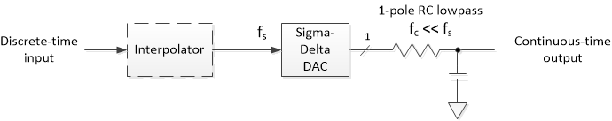
Figure 1.  Sigma-Delta DAC with one-pole RC lowpass filter.

f_s = SD DAC sample rate; f_c = RC filter -3 dB bandwidth.

Example 1.

A simple example is shown in Figure 2.  The discrete-time input signal is plotted in the top of Figure 3 (the individual samples blur together).  The signal is unsigned with a level range of 0 to 1.  The sample rate is 1 MHz, and the RC filter values are 4700 ohms and .01 μF.  Here is the Matlab code to compute the one-bit discrete-time output y and the analog output y_filt:

    R= 4.7e3;                 % ohms resistor value
    C= .01e-6;                % F capacitor value
    fs= 1e6;                  % Hz DAC sample rate
    % input signal
    x= [zeros(1,20) .9*ones(1,200) .1*ones(1,200)];
    % find output y of SD DAC and output y_filt of RC filter
    [y,y_filt]= sd_dacRC(x,R,C,fs);

The SD DAC output y is shown in the middle plot of Figure 3, and the bottom plot is the output y_filt of the RC filter.  Note the changes in y that coincide with the amplitude steps in x (near n = 20 and n = 220).  The exponential rise and fall of y_filt is due to the RC filter portion of the model.  Figure 4 shows x and y_filt for the case of a longer pulse:

    x= [zeros(1,100) .9*ones(1,1500) .1*ones(1,1000)];

Again, the individual samples of x cannot be distinguished in the plot.  In both Figures 3 and 4, there is noise visible on the RC filter output signal; this is the remaining SD DAC quantization noise after filtering.

The Matlab function also computes the RC -3 dB frequency as approximately 3.39 kHz:  fc = 3.3863e+03.  This gives us a ratio of f_s/f_c of 1E6/3.39E3 ≈ 295.  The SD DAC can be used for lower ratios of f_s/f_c, but may require a higher-order lowpass filter (often implemented as an active filter).

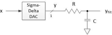
Figure 2.  SD DAC with one-pole RC filter.

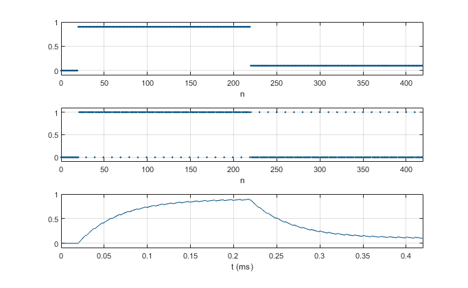
Figure 3. Time response of SD DAC plus RC filter.  f_s = 1 MHz, R = 4.7 KΩ, C = .01 μF                     (f_c = 3.39KHz).

Top:  Discrete-time input signal x.   Center:  SD DAC output y.   Bottom: RC filter output y_filt.

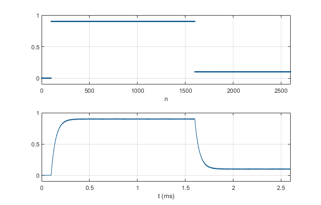
Figure 4.  Time Response for a longer pulse.  Same f_s and RC as used in Figure 3.

Top:  Discrete-time input signal x.   Bottom:  RC filter output y_filt.

SD DAC Basic Operation

A first-order SD DAC is simply a binary accumulator with a carry output, as shown in Figure 5a.  The one-bit output y(n) is the carry output of the adder.  Figure 5b shows an equivalent block diagram.  Here mod(u,1) computes s = u, modulo 1.

Suppose we apply a constant input C, where 0 <= C < 1.   Figure 6 shows the sum s(n) and carry y(n) for C = 5/32.  y(n) equals 1 each time s(n) rolls over.  On average, there are 1/C samples per rollover period of y(n):

$$ avg. rollover \; period = \frac{modulus}{C}= \frac{1}{C} \qquad (1) $$

For this example, 1/C = 32/5 = 6.4 samples, and the rollover period varies between 6 and 7 samples.  Given N samples of y(n), the number of 1’s is the sum of all y values, which is given by:

$$ \sum_{n=0}^{N-1}y(n) \approx \frac{N}{avg. rollover \; period} = NC \qquad (2) $$

Thus,

$$ \frac{\sum y(n)}{N} \approx C \qquad (3) $$

That is, the average value of y(n) is approximately C.  We can approximate C by filtering y(n) with a lowpass filter having f_c << f_s, as shown in Figure 2.  Furthermore, if we allow x(n) to vary slowly, the output of the lowpass filter will approximate x(n) if the bandwidth of x(n) is less than f_c.

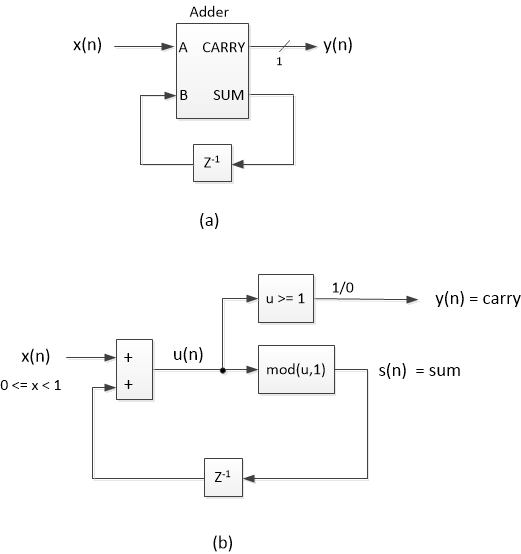
Figure 5.  a) SD DAC binary implementation.  b) Equivalent block diagram.

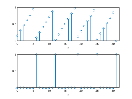
Figure 6.  SD DAC signals for constant input = 5/32.   Top:  s(n).   Bottom:  y(n).

Quantization Noise Shaping of the SD DAC

The quantization error of y(n) in figure 5b is:

$$ e(n)= y(n)-u(n) \qquad (4)$$

The quantity s(n) is equal to the negative of the quantization error:

$$ s(n) = -e(n) \qquad (5) $$

For example, if u(n) = 11/8, then y(n) = 1 and s(n) = mod(11/8,1) = 3/8.  The quantization error from Equation 4 is e = 1 – 11/8 = -3/8.  (Note that the top plot of Figure 6 is s(n) = -e for constant x = 5/32).

Using Equations 4 and 5, we can create a SD DAC block diagram that is equivalent to Figure 5b, as shown in Figure 7 [1,2].  From this figure, we see that:

$$ u(n) = x(n) - e(n-1) \qquad (6) $$

Substituting this expression for u(n) in (6) into (4), and rearranging, we get:

$$ y(n) = x(n) + e(n) - e(n-1) \qquad (7) $$

So, the output is equal to the input plus the difference of the current and previous quantization error samples.  From Equation 7, the SD DAC’s transfer function for quantization error (quantization noise) is:

$$ G(z)= 1 - z^{-1} \qquad (8) $$

We recognize G(z) as a first-difference differentiator.  The frequency response magnitude |G(f)| can be plotted using the following Matlab code:

    b= [1 -1];          % G(z) coeffs
    N = 512;            % dft length
    [G,f]= freqz(b,1,N,1);
    Gmag= abs(G);       % magnitude response

The resulting magnitude response is shown in Figure 8 (top), where we see that the noise is attenuated at low frequencies and amplified at high frequencies. The bottom of Figure 8 plots Gmag in dB using a log frequency scale.  The quantization noise is attenuated approximately 30 dB for f/f_s = .005 = 1/200.

Keep in mind that the quantization noise of the one-bit quantizer is shaped by G(f); the noise spectrum of the quantizer itself is rather unpredictable, because quantization is a non-linear process.  The overall noise spectrum depends on the signal applied to the SD DAC as well as on G(f).  Some interesting SD DAC spectra are provided in [3].

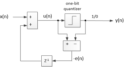
Figure 7.  SD DAC block diagram equivalent to Figure 5b.

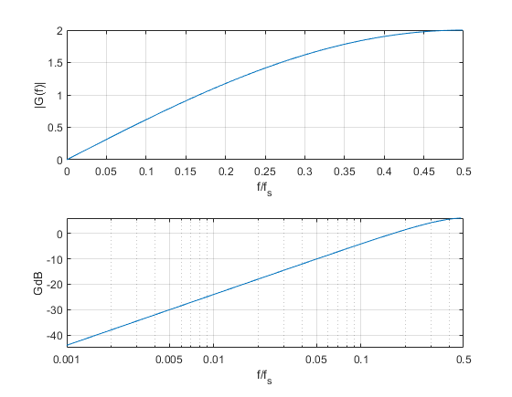
Figure 8.  Magnitude response of SD DAC for quantization noise.

Top:  linear scales.   Bottom:  log frequency scale and dB amplitude scale.

Matlab Function sd_dacRC

Now we’re ready to create our SD DAC model.  The Matlab function for modeling the system of Figure 2 is listed below.  The model first quantizes the input x to 16 bits.  It then implements the system of Figure 5b.  The model includes a one-pole IIR filter to approximate the response of the RC lowpass.  The IIR filter has transfer function:

$$ H(z)= \frac{b_0}{1+a_1z^{-1}}  \qquad (9) $$

Appendix A in the PDF version derives formulas for the filter coefficients from R, C, and f_s.  Note that the function prints the value of f_c to the workspace (by not terminating the expression for f_c with a semicolon).  The model treats the digital buffer feeding the RC filter as an ideal switched voltage source.  The value of R should typically be greater than 1000 ohms, assuming 3.3 volt logic levels.

Finally, we consider whether the SD DAC model should include a zero-order hold (ZOH) function [4] for accurate computation of the spectrum.  Given that the cut-off frequency f_c of the RC lowpass filter is much less than f_s, the sinx/x roll-off of the response at f_c is small and the ZOH need not be modeled.  However, to estimate the quantization noise spectrum up to f_s/2 or above, we would need a ZOH model.  We’ll discuss adding a ZOH model later in this article.

Disclaimer:  The author believes this code to be correct, but it may contain errors. Do not use the results without verifying them.

    % function [y,y_filt] = sd_dacRC(x,R,C,fs)  2/5/24 Neil Robertson
    % 1-bit sigma-delta DAC with RC filter
    % Model does not include a zero-order hold.
    %
    % x = input signal vector, 0 <= x < 1
    % R = series resistor value, Ohms.  Normally R > 1000 for 3.3 V logic.
    % C = shunt capacitor value, Farads
    % fs = sample frequency, Hz
    % y = DAC output signal vector, y(n) = 0 or 1
    % y_filt = RC filter output signal vector
    %
    function [y,y_filt] = sd_dacRC(x,R,C,fs)
    N= length(x);
    x= fix(x*2^16)/2^16;        % quantize x to 16 bits
    %I 1-bit Sigma-delta DAC
    s= [x(1) zeros(1,N-1)];
    for n= 2:N
        u= x(n) + s(n-1);
        s(n)= mod(u,1);        % sum
        y(n)= fix(u);          % carry
    end
    %II One-pole RC filter model
    Ts= 1/fs;
    Wc= 1/(R*C);               % rad -3 dB frequency
    fc= Wc/(2*pi)              % Hz -3 dB frequency
    a1= -exp(-Wc*Ts);
    b0= 1 + a1;                % numerator coefficient
    a= [1 a1];                 % denominator coeffs
    y_filt= filter(b0,a,y);    % filter the DAC's output signal y

Example 2.  Sinewave

This example applies a sinewave with frequency f₀ = 999 Hz to an SD DAC clocked at 1 MHz.  We consider two cases for the RC filter:  .01 uF/1500 ohms and .01 uF/4700 ohms.  Here is the Matlab code to generate the sinewave and compute the outputs for the two cases:

    fs= 1e6;             % Hz DAC sample rate
    Ts= 1/fs;
    f0= 999;             % Hz sinewave frequency
    A= .9;               % sinewave amplitude
    N= 2^14;             % number of samples
    n= 0:N-1;            % sample index
    x = A*sin(2*pi*f0*n*Ts);     % input signal
    x= .5*(x + 1);        % convert signed to unsigned (invert MSB)
    % RC filter case 1
    C= .01e-6;            % F capacitor value
    R1= 1.5e3;            % ohms resistor value
    [y,y_filt1]= sd_dacRC(x,R1,C,fs);
    % RC filter case 2
    R2= 4.7e3;            % ohms resistor value
    [y,y_filt2]= sd_dacRC(x,R2,C,fs);

Figure 9 plots the RC filter output sinewave for the two filter cases.  You can see quantization noise on the .01 uF/1500 ohm case (top plot), which has f_c = 10.6 kHz.  The noise is attenuated further in the bottom plot, with RC = .01 uF/4700 ohm and f_c = 3.4 kHz.

In computing the spectrum of the output y_filt, our model has two main sources of error:  first, it does not compute the sinx/x spectrum roll-off caused by the SD DAC’s zero-order hold (ZOH); and second, there is error in the magnitude response of the RC filter model at higher frequencies.  We can reduce both errors by adding a ZOH model [4].  The Matlab function sd_dacRCzoh, which is listed in Appendix B of the PDF version, includes a ZOH model.  The output signal vectors of sd_dacRCzoh have a sample rate of 4 times that of the input signal vector x.

In the above code, we can replace the function calls to sd_dacRC with the following calls, and compute the spectra of the output signals (removing the dc component):

    [y_zoh,y_filt1]= sd_dacRCzoh(x,R1,C,fs);
    [y_zoh,y_filt2]= sd_dacRCzoh(x,R2,C,fs);
    y_zoh= 2*y_zoh-1;               % convert unipolar to bipolar (remove dc)
    y_filt1= 2*y_filt1-1;
    y_filt2= 2*y_filt2-1;
    % compute spectra
    [PdB1,f]= psd_kaiser(y_zoh,4*N,4*fs);
    [PdB2,f]= psd_kaiser(y_filt1,4*N,4*fs);
    [PdB3,f]= psd_kaiser(y_filt2,4*N,4*fs);

The function psd_kaiser is listed in Appendix C of the PDF version.  The output spectrum of the SD DAC with ZOH is shown in the top plot of Figure 10, where we see the shaping of the quantization noise spectrum predicted by Equation 8 and Figure 8.  The spectral null at f_s = 1 MHz is caused by the ZOH.  The middle and bottom plots of Figure 10 show the effect of the RC filter upon the spectrum, for two values of f_c.

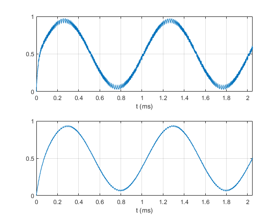
Figure 9.  Example 2:  sinewave at 999 Hz, f_s = 1 MHz.

Top:  RC output for f_c = 10.6 kHz.    Bottom:  RC output for f_c = 3.4 kHz.

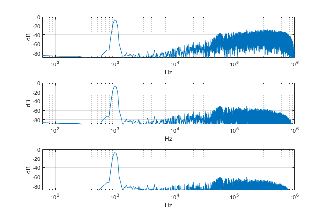
Figure 10.  Spectra of SD DAC output signals for Ex. 2, with ZOH.  f₀ = 999 Hz, f_s = 1 MHz.

Top:  SD DAC ZOH output.   Middle:  RC output for f_c = 10.6 kHz.   Bottom:  RC output for f_c = 3.4 kHz.

Example 3.  DC signal

We can apply a constant (DC) signal to the SD DAC model and compute the outputs as follows:

    fs= 1e6;              % Hz DAC sample rate
    R= 4.7e3;             % ohms resistor value
    C= .01e-6;            % F capacitor value
    % input signal
    A1= .925;
    N= 1024;
    x1= A1*ones(1,N);     % constant input vector
    [y1,y_filt1]= sd_dacRC(x1,R,C,fs);

The output signal is shown in Figure 11, along with the outputs for other DC input levels.  The RC filter has f_c = 3.4 kHz.  In all cases, the output quantization noise appears as a periodic pattern with a spectrum containing a tone and harmonics [2].  For example, the spectra for x = 0.925 are computed as follows:

    y1= 2*y1- 1;            % convert unipolar to bipolar
    y_filt1= 2*y_filt1- 1;
    [YdB,f]= psd_kaiser(y1,N,fs);
    [Yfilt_dB,f]= psd_kaiser(y_filt1,N,fs);

(Since we are not concerned about spectrum amplitude accuracy at high frequencies, we did not use the function that includes the SD DAC zero-order hold).  The spectrum at the SD DAC output is shown in the top of Figure 12, and the spectrum of the RC filter output is shown in the bottom.  The quantization noise spectra don’t resemble the “noise-like” ones for the sinewave of Example 2.

Note that the fundamental tone of the quantization noise spectrum is only 25 kHz.  To attenuate the quantization noise further, we could lower f_c, increase f_s, or use a higher order analog filter.

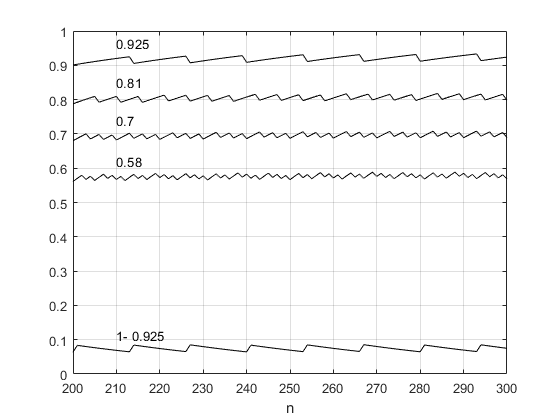
Figure 11.  SD DAC outputs for constant input values as indicated on plot, f_c = 3.4 kHz, f_s = 1 MHz.

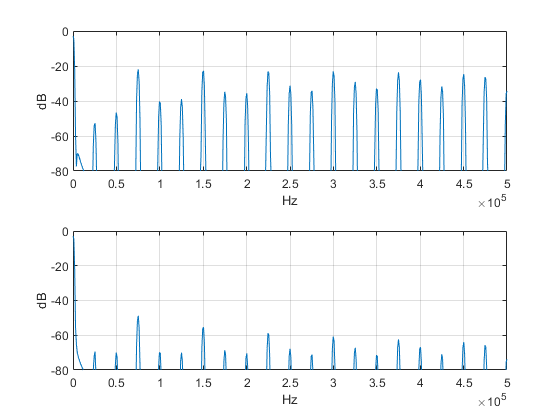
Figure 12.  Top:  Spectrum of SD DAC output for constant input x = 0.925, f_s = 1 MHz.

Bottom:  Spectrum of RC output, f_c = 3.4 kHz.

Conclusion

We have seen how to create a model that combines a basic SD DAC with a one-pole RC low-pass filter.  The model allowed us to evaluate the time domain and frequency domain performance vs f_s and the element values (or equivalently, f_c) of the filter.  In all cases, we used a very high f_s compared to the filter f_c.  This high sample frequency was needed because of the low selectivity of the one-pole RC filter.  We could reduce the sample frequency relative to f_c by using a higher-order analog filter.

See the PDF version for Appendices.

References

1.  Mitra, Sanjit K., Digital Signal Processing, A Computer-Based Approach, 2^nd Ed., McGraw Hill, 2001, p 822 – 826.

2.  Pavan, Shanthi, Richard Schreier, and Gabor C. Temes, Understanding Delta-Sigma Data Converters, 2^nd Ed., Wiley, 2017, Ch. 1 and 2.

3.  Sachs, Jason, “Return of the Delta-Sigma Modulators, Part 1 : Modulation", DSPRelated.com, May, 2023, https://www.dsprelated.com/showarticle/1517/return-of-the-delta-sigma-modulators-part-1-modulation

4.  Robertson, Neil, “DAC Zero-Order Hold Models”, DSPRelated.com, Jan, 2024, https://www.dsprelated.com/showarticle/1627.php

5.  Robertson, Neil, “A Simplified Matlab Function for Power Spectral Density”, DSPRelated.com, March, 2020, https://www.dsprelated.com/showarticle/1333.php

Neil Robertson      March, 2024

Sign in