Digital PLL's -- Part 2

• Matlab
• Tutorials

In Part 1, we found the time response of a 2^nd order PLL with a proportional + integral (lead-lag) loop filter.  Now let’s look at this PLL in the Z-domain [1, 2].  We will find that the response is characterized by a loop natural frequency ω_n and damping coefficient ζ. 

Having a Z-domain model of the DPLL will allow us to do three things:

1. Compute the values of loop filter proportional gain K_L and integrator gain K_I that give the desired loop natural frequency and damping.  Deriving these formulae is somewhat involved, but the good news is we only have to do it once.
2. Compute the linear-system time response to a step in the reference phase.
3. Compute the frequency response.

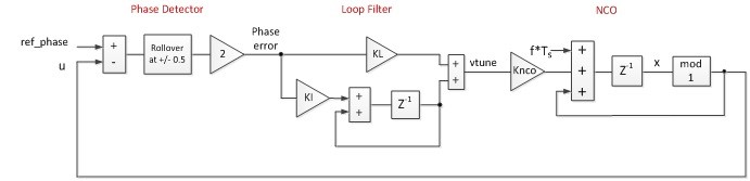
Figure 1.  DPLL Time Domain Model Block Diagram

Figure 1 is the time-domain DPLL model we derived in part 1.  To convert this to a useful Z-domain model, we replace the accumulators in the Loop Filter and NCO with the transfer function  z^-1/(1 – z^-1), who’s numerator and denominator we can multiply by z to get 1/(z – 1).  This gives us the model in Figure 2, where we have also indicated the phase detector gain K_p.

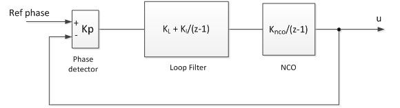
Figure 2.  DPLL in the Z-domain

The open-loop response of this system is the product of the transfer functions of the three blocks:

$$ G_1(z) = \frac{K_pK_LK_{nco}}{z-1} + \frac{K_pK_IK_{nco}}{(z-1)^2} \tag{1}   $$                   

2^nd Order System in s and z

A 2^nd order continuous-time system with a Lead-lag filter is shown in Figure 3. [3, 4].  See Appendix B for a derivation of the closed-loop response.  If we convert this to the Z-domain, we’ll see the response has the same form as that of our DPLL.  This will allow us to relate K_L and K_I of the DPLL to ω_n and ζ.

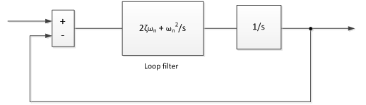
Figure 3.  2^nd order system in s with a zero in the closed-loop response

To convert this system to the z-domain equivalent, make the following replacement:

      $$ s \rightarrow \frac{z-1}{T_s} $$

This approximation is valid as long as the loop natural frequency is much less than the sample frequency (see Appendix C).  The Z-domain block diagram is shown in Figure 4, where we have allowed for the possibility that the loop filter could have a sample rate T_{s_filt}  different from the NCO sample rate T_{s_nco}.

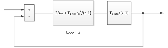
Figure 4.  2^nd order system in the z-domain

The open-loop response G₂(z)  is:

$$ G_2(z) = \frac{2\zeta\omega_nT_{s\_nco}}{z-1} + \frac{T_{s\_filt}T_{s\_nco}\omega_n^2}{(z-1)^2} \tag{2} $$

By equating open-loop response G₁ of our DPLL to G₂, we can find K_L and K_I in terms of ω_n and ζ. 

Equating G₁ and G₂:

$$ \frac{K_pK_LK_{nco}}{z-1} + \frac{K_pK_IK_{nco}}{(z-1)^2} = \frac{2\zeta\omega_nT_{s\_nco}}{z-1} + \frac{T_{s\_filt}T_{s\_nco}\omega_n^2}{(z-1)^2} $$   

Solve for K_L and K_I:

  $  K_pK_LK_{nco} = 2\zeta\omega_nT_{s\_nco} $        →        $ K_L = 2\zeta\omega_n/K_p\; * \; T_{s\_nco}/K_{nco} $          (3)

  $ K_pK_IK_{nco} = T_{s\_filt}T_{s\_nco}\omega_n^2 $      →     $ K_I = T_{s\_filt}\omega_n^2/K_p \; * \; T_{s\_nco}/K_{nco} $          (4)

A given DPLL design has defined values for T_{s_filt},T_{s_nco}, K_p, and K_nco.  Given those values, K_L and K_I are uniquely determined by the choice of ω_n and ζ.    Note that the units of K_p are cycle^-1.  See Appendix D for an alternate form of the equations for K_L and K_I.

Computing the Closed-loop response

The closed loop phase response of the DPLL in Figure 2 is given by:

$$ CL(z) = \frac{Z[u]}{Z[ref\_phase]} = \frac{G_1}{1 + G_1}   $$

Thus from equation 1,

       $$ \frac{K_pK_LK_{nco}} {z-1} + \frac{K_pK_IK_{nco}} {(z-1)^2}   $$

           $ CL(z) = $                       __________________________________

             $$ 1 + \frac{K_pK_LK_{nco}} {z-1} + \frac{K_pK_IK_{nco}} {(z-1)^2}   $$  

$$ CL(z) = \frac {b_0 + b_1z^{-1}} {1 + a_1z^{-1} + a_2z^{-2}}    \qquad        (5)   $$   

Where

b₀ = K_pK_LK_nco
b₁ = K_pK_IK_nco - K_pK_LK_nco
a₁ = K_pK_LK_nco – 2
a₂ = 1 + K_pK_IK_nco - K_pK_LK_nco

Equation 5 is in the form of an IIR filter transfer function, which allows for straightforward computation of the time and frequency responses in Matlab.

Example

This example uses the same parameters as Example 2 in Part 1.  We will compute K_L and K_I, then we will find the time and frequency response using CL(z).  For this example, f_{s_nco} = f_{s_filt} = f_s.  The Matlab script is listed in Appendix A.   The DPLL parameters are as follows.  As you can see, not all of the parameters from the time domain model apply to the Z-domain model.

f_s                                                  25 MHz
Reference frequency                   NA
Initial reference phase                 NA
NCO initial frequency error          NA
K_nco                                             1/4096
K_p                                                2 cycle^-1
f_n                                                 400 Hz   loop natural frequency.  f_n = ω_n/(2π)
ζ                                                  1.0           loop damping coefficient

1.  Find K_L and K_I

KL= 2*zeta*wn*Ts/(KP*Knco)      % loop filter proportional gain
KI= wn^2*Ts^2/(KP*Knco)         % loop filter integral gain
    KL = 0.4118
    KI = 2.0698e-005

2.  Compute the time response to a step in the reference phase.  Since CL(z) is in the form of a digital filter transfer function, we can find the time response using the Matlab "filter"  function.

b0= KP*KL*Knco;
b1= KP*Knco*(KI - KL);
a1= KP*KL*Knco - 2;
a2= 1 + KP*Knco*(KI - KL);
b= [b0 b1];         % numerator coeffs
a= [1 a1 a2];       % denominator coeffs
x= ones(1,N);       % step function
y= filter(b,a,x);   % step response
pe= y-1;            % phase error response

The phase error response is shown in Figure 5.  Because this model is linear, the non-linear acquisition behavior we saw in the time-domain model of Part 1 (Figure 3.4) is missing.  Thus we see that the Z-domain model is less capable than the time-domain model for computing the time response.  Finally, one detail worth mentioning:  the response has some overshoot.  This is caused by the zero in CL(z).  (An all-pole system would not have overshoot for ζ = 1). 

3.  Compute the frequency response CL(z).

u = 0:.1:.9;
f= 10* 10 .^u;                  % log-scale frequencies
f = [f 10*f 100*f 1000*f];
z = exp(j*2*pi*f/fs);           % complex frequency z
CL= (b0 + b1*z.^-1)./(1 + a1*z.^-1 + a2*z.^-2);  % closed-loop response
CL_dB= 20*log10(abs(CL));
semilogx(f,CL_dB),grid

The closed-loop frequency response is shown in Figure 6.  Comparing this response to that of the equivalent continuous-time system in Figure B.2, we see that they match.  Note the peak in the response occurs near the loop natural frequency of 400 Hz.  The slope of the response in the stopband is -20 dB/decade.

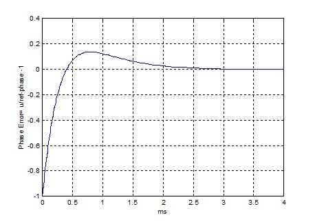
Figure 5.  Phase Error for unit-step change in reference phase.  f_n = 400 Hz, ζ = 1.0.

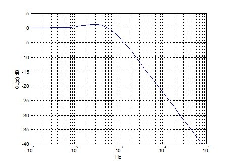
Figure 6.  Closed-Loop Frequency Response.  f_n = 400 Hz, ζ = 1.0.

4.  Plot the step response and the frequency response for different values of damping.  Figure 7 shows the step response and Figure 8 shows the frequency response.

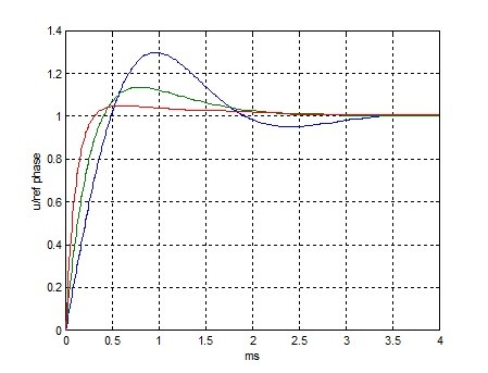
Figure 7.  Step Response.  f_n = 400 Hz;  ζ = 0.5 (blue), 1.0 (green), 2.0 (red)

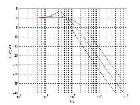
Figure 8.  Closed-Loop Frequency Response.  f_n = 400 Hz;  ζ = 0.5 (blue), 1.0 (green), 2.0 (red)

Appendix A.  Z-Domain model of DPLL with f_n = 400 Hz

%pll_response_z2.m     nr  5/24/16
% Digital 2nd order type 2 PLL
% step response and closed loop frequency response
Knco= 1/4096;       %   NCO gain
KP= 2;              % 1/cycles  phase detector gain
wn = 2*pi*400;      % rad/s   loop natural frequency
fs = 25e6;         % Hz sample rate
zeta = 1;           % damping factor
Ts= 1/fs;           % s  sample time
KL= 2*zeta*wn*Ts/(KP*Knco)      % loop filter proportional gain
KI= wn^2*Ts^2/(KP*Knco)         % loop filter integral gain
% Find coeffs of closed-loop transfer function of u/ref_phase
% CL(z) = (b0 + b1z^-1)/(a2Z^-2 + a1z^-1 + 1)
b0= KP*KL*Knco;
b1= KP*Knco*(KI - KL);
a1= KP*KL*Knco - 2;
a2= 1 + KP*Knco*(KI - KL);
b= [b0 b1];         % numerator coeffs
a= [1 a1 a2];       % denominator coeffs
% step response
N= 100000;
n= 1:N;
t= n*Ts;
x= ones(1,N);       % step function
y= filter(b,a,x);   % step response
pe = y – 1;         % phase error response
plot(t*1e3,pe),grid
xlabel('ms'),ylabel('Phase Error = u/ref-phase -1'),figure  %plot phase error
% Closed-loop frequency response
u = 0:.1:.9;
f= 10* 10 .^u;                  % log-scale frequencies
f = [f 10*f 100*f 1000*f];
z = exp(j*2*pi*f/fs);           % complex frequency z
CL= (b0 + b1*z.^-1)./(1 + a1*z.^-1 + a2*z.^-2);    % closed-loop response
CL_dB= 20*log10(abs(CL));
semilogx(f,CL_dB),grid
xlabel('Hz'),ylabel('CL(z) dB')

Appendix B.  2^nd order continuous-time system closed loop response in s

Figure B.1.  2^nd order system in s with a zero in the closed-loop response

$ A(s) = 2\zeta\omega_n + \frac {\omega_n^2} {s}  $        lead-lag filter

$  G(s) = \frac {1} {s} A(s)  = \frac {2\zeta\omega_n} {s}  + \frac {\omega_n^2} {s^2}$

$CL(s) = G/(1+G) $

$ CL(s) = \frac {2\zeta\omega_n + \omega_n^2} {s^2 + 2\zeta\omega_n + \omega_n^2} $

where

ω_n= 2πf_n = loop natural frequency
ζ= damping factor

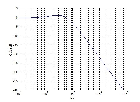
Figure B.2.  Closed-Loop Frequency Response.  f_n = 400 Hz, ζ = 1.0. 

Appendix C.  Converting H(s) to H(z)

This is a way to approximate H(s) when a system’s passband frequency range is much less than the sample frequency.  We choose this method because it results in a block diagram and transfer function that have the same form as that of our DPLL in Figure 2. 

The definition of z is:

z = exp(sT_s)                        

where s is complex frequency and T_s is the sample time.  If we approximate z by the first two terms in the Taylor series for e^x, we have

z ~= 1 + sT_s                  (1)

Here we are assuming 2πfT_s  << 1, or f/f_s << 1/2π.  For our examples, we have been using f_n = 5 kHz or less and fs = 25 MHz.  So f_n/f_s = .0002 << 1/2π.

Rearranging equation 1, we get

s ~= (z – 1)/T_s

To convert H(s) to H(z) we replace each occurrence of the variable s by (z – 1)/T_s. 

Appendix D.  Alternative formulae for loop filter coefficients

The gain block in front of the NCO has gain Knco.  The output frequency of the NCO due just to Vtune is

f   = Vtune*K_nco*f_{s_nco}

If we define K_v = K_nco*f_{s_nco}        Hz,

then K_nco can be replaced by K_v*T_{s_nco} in the formulae for K_L and K_I.  So equations 3 and 4 become:

$ K_L = 2\zeta\omega_n/(K_pK_v)  $

$ K_I = \omega_n^2T_{s\_filt}/(K_pK_v) $

Here, the units of K_p are cycle^-1, which is consistent with K_v in Hz.  Alternative units for K_p and K_v are radian^-1 and rad/s, respectively.

References

1.  Gardner, Floyd M., Phaselock Techniques, 3^rd Ed., Wiley-Interscience, 2005, Chapter 4.

2.  Rice, Michael, Digital Communications, a Discrete-Time Approach, Pearson Prentice Hall, 2009, Appendix C.

3.  Gardner, Section 2.2.3.

4.  Rice, C.1.3

6/9/2016            Neil Robertson

Sign in