Dear all,

I am trying to confirm Nyquist-Shannon theorem through matlab-simulink.

More particular I am trying to confirm what would be the minimum achievable sampling rate for a given M-PSK waveform. In a real scenario the detected signal of certain bandwidth Y would be reaching the ADC in its continuous time form.Theoretically the ADC would have to sample at a rate 2xY for that signal to be recovered properly after digitization.

In a simulation environment the waveform is being generated "digitally" meaning that is effectively a set of samples at a particular rate.The BW of that signal is being plotted using FFT under the assumption that in the far ends of the spectrum frequencies of half the sampling rate will appear.

How will one confirm the Nyquist-Shannon theory given the above?

If one tries to "select" some of those samples (try to approximate the behavior of an ADC,with no quantization noise applied) will introduce down-sampling. That will have dissimilar effects to the ones introduced by ADC sampling on a ct waveform (and most likely interpolation will be also necessary on the other end). 

What  is the way usually followed to confirm the theory given the above?

Could you please provide some pointers?

G

"How will one confirm the Nyquist-Shannon theory given the above?"

Forgive me if English is not your native language, but there's a terminology issue here.  It's not clear what you mean by "confirm".  If you mean "prove" using simulation -- no, you can't.  Mathematical theorems, like Nyquist-Shannon, are proven using logic, symbolically.  A simulation can only cover one case.  If you mean "demonstrate", then yes, you can demonstrate specific examples, but you cannot make an overall proof.

As a counterexample, consider a signalling system that encodes $n$ bits into $M = 2^n$ symbols, where each symbol is a perfect rectangle $T$ seconds long and takes the value $e^{j 2 \pi k/M}$, where $k \in [0, M)$ and the values of $k$ are randomly chosen.

The signal will have infinite bandwidth (its spectrum, if I'm getting the constants right, will be $\frac{sin \omega T}{\omega T}$).  But if you sample at the center of each symbol, then in the absence of noise you'll have perfect reception.

This counterexample is not the only one -- there are whole families of signals that fall into this general category.  There is theory that pertains to this, but it's not the Shannon-Nyquist sampling theorem.

My suggestion is that if you're ready to get away from cookbook explanations of Nyquist-Shannon (like mine, shameless plug: https://www.wescottdesign.com/articles/Sampling/sampling.pdf) that you either carefully read the modern literature on the subject, or that you look at communication's theory's two founding papers by Shannon.  They're references 1 and 2 for this paper: http://www.hit.bme.hu/~papay/edu/Conv/pdf/origins.pdf and if you search on the titles you'll find them.

You'll need to understand the Fourier transform in and out, and how to model sampling as multiplication as a train of dirac impulses, but if you can do that and if you work at it you should be able to follow the proof.

Then, having really proved it to yourself, you won't have to depend on inherently unreliable demonstrations.

(I can't seem to get MathJax working today.  I'm leaving this stand for now, though).

Thank you very much for your answer!Sorry for the confusion that my English has created.

I am trying to provide some clarity on what would be the minimum sampling rate for an M-PSK waveform generated in Matlab/simulink.To be more precise random numbers are being "mapped" by a Matlab library to M-PSK complex symbols.Then those symbols are being passed through a RRC interpolation filter.The rate that the random numbers are generated and the interpolation factor are effectively defining the sample rate.However that sequence of symbols is where I need to consider "continuous time" and prove that if I sample Bellow a certain rate I wont be able to recover the information.That is the reason why I have used the name Nyquist.Forgive me if that was not very accurate

You keep using "prove" in the same statements with Matlab.  In other words, you're asking how to prove something using experimental mathematics.

You can use experimental mathematics to prove that a particular solution to a problem exists (by solving it).  But that solution using experimental mathematics only defines one point in a problem space with many, possibly infinite dimensions.

You cannot make general proofs using experimental methods in mathematics.  And there's a proof for it -- in informal terms, to do so would be the same as filling in a continuous multidimensional space with a finite number of points -- and there's a pretty easy proof of why that's impossible even just on a line segment, much less a multidimensional space.

So -- Matlab or real life, if you have a well-formed signal for which the timing is known then the minimum effective sampling rate is exactly once per symbol.  This is well known from theory.  Life gets more difficult if you need to recover carrier and bit timing -- the typical number quoted is twice the symbol timing, but just off the top of my head I can think of ways to do this with less if you allow me irregular sampling.

There's a name for the condition you need to impose on the signal that makes it well-formed enough for that "once per symbol" conclusion to hold, but I can't remember it off the top of my head -- but the important part about it is that it takes half a page to prove mathematically, if you have the background, and you would never, ever be able to prove it experimentally because of that whole "fill a continuous space with a finite number of points" problem.

Very helpful,thank you so much!

At Tx you need two samples per symbol minimum. Why? for shaping because if you send symbols in air without shaping the bandwidth you will get in trouble with law affecting a wide spectrum. That is why you use RRC to shape the bandwidth.

In air the information part of your signal is actually every other sample (your symbols). At Rx you will naturally receive that signal. You then exploit the two samples per symbol before downsampling to one sample per symbol.

There is no need to prove what is already proven regarding Nyquist rule at ADC. That requires proper time dimension which does not exist in Matalab.

Thank you for your answer!

Is there a compelling reason why you want to prove the theorem with M-PSK signal?

It is far easier to prove the theorem using a simple sine wave that is close to half the sample rate, and then interpolate (digitally) down from there to show how the spectrum folds around the Fs/2 frequencies.

Thank you very much for your repky,yes a M-PSK waveform is the requirement.Since we talk about a communication system that would run using M-PSK.

It will depend very much on the waveform that you are using (or generating). If, for instance, you have square-wavelike behavior, your Fourier transform will present a Gibbs phenomenon at the corners; the same will be true at any discontinuity of the waveform. You can minimize the phenomenon by adding more terms, but never get rid of it.

You are also assuming that the ADC is ideal, which is usually not. Any filtering introduced by the ADC will require for some oversampling above the Nyquist frequency. The same is true if the signal is digitally generated.

You can try to confirm the Nyquist theorem by using as-clean-as-possible ADC simulators and well behaved signals, in a very long time interval (the idea of reconstructing via FT applies to perfectly periodic signals; once your time interval is bounded the signal can no longer be seen as periodic).

Thank you very much for your reply.Consider simply that I have a Matlab library "mapping" random numbers to M-PSK symbols.Those random numbers are generated at a certain rate which effectively defines the sampling rate of the system.Then those symbols are passed through an interpolation RRC.After that is the point that I would need to prove Nyquist theorem.So effectively, I need to prove that "sampling" that waveform Bellow a certain rate would effectively render it unrecoverable.And that rate I assume that would be the Nyquist rate?The confusing bit is that the waveform is already discrete so we can talk only about downsampling?

If a matched filter is applied and the sample timing is synchronized to the symbols, you only need one sample per symbol to fully recover M-PSK. 

Only one sample per symbol even for non BPSK waveforms?

That is correct, any M-PSK or M-QAM or M-ASK signal requires only one (complex) sample per symbol to recover the information.   Again, this assumes that a matched filter is applied (e.g., a matching RRC filter), and the sample timing is synchronized to the symbols centers.

Here is a Simulink model that can be used to answer your question.

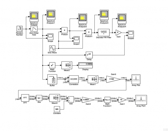
Random numbers between -1 and +1 with a period of 1/100 s are generated from a Random Number block. These can be viewed as in-phase components for an M-PSK or Q-PSK.

With the Zero-Order Hold block, will these components scanned at 10000 Hz, so that 100 identical values occur in each period.

The in-phase carrier for the modulation must then have a frequency between 0 and 10000/2 = 5000 Hz. A carrier frequency of 1000 Hz was selected in the model

The demodulator is simulated with the same carrier. The double frequency is suppressed with the FIR filter from the Block Discrete FIR Filter.

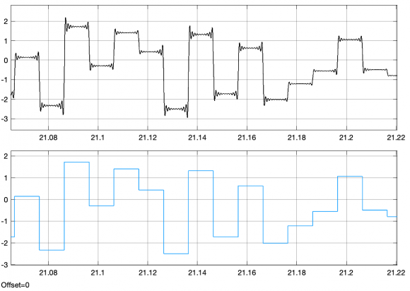
The demodulated sequence is shown on the Scope 2 block together with the input signal.

On the Spectrum Analyzer blocks (at the top) you can observe the PSD at various points in the model.

The average power of the input signal is determined in the model and shown on the display block.

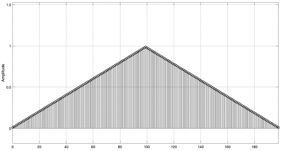
In the model, the PSD is also determined from the autocorrelation and displayed in the lower part. With the zoom function, the same PSD can be viewed as shown on the Spectrum Analyzer1.

The autocorrelation shown on Array Plot block is:

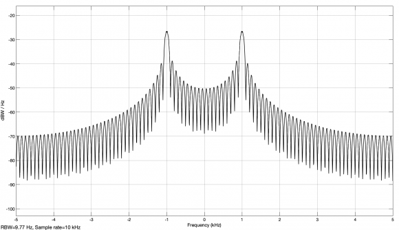
The PSD of the modulated Signal, as it is shown on Spectrum Analyser2 block is:

The Simulink model M_PSK_2.slx

M_PSK_2.slx