Hello,

There is probably an easier way to do this, but I am getting stuck on trying to determine the following FIR filter design.

Let's suppose that I have a transfer function that is H(w). This transfer function is a a 1x512 point vector in matlab. My question is, how do I get the discrete time signal h(n) from this vector H(w)?

Here is what I have (unsuccessfully) tried:

So I know that the DFT of X(w) is, x(k) = X(2*pi*k/N).

then in h(n) = ifft(X(2*pi*k/N)) which would be FIR coefficients. so in matab:

h is my h(n), discrete time signal

H is my H(w), Discrete Time Fourier Transform (DTFT)

h=ifft(H(1:2*pi/N:end) );  %this does not seem to produce good results.

Is there a better way to scale H(w) to get the DFT h(k)? Any recommendations?

Thanks :D

Hi,

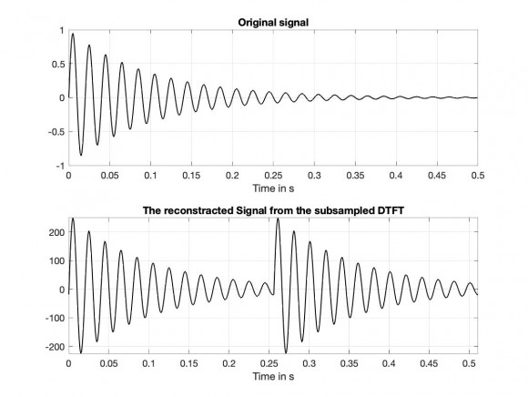
i think you have a time aliasing due to the sampling of the DTFT and therefore the reconstructed signal via the inverse DTFT is not the expected signal.

With the following MATLAB script you can understand that.

The DTFT is initially approximated with nfft = 512 samples via the DFT. The DTFT is then subsampled with M <nfft samples. The reconstructed signal is then calculated from these samples using an inverse DTFT:

xr (ni) = sum (Xr * exp (j * 2 * pi * (ni-1) * (0: M-1) / M));

ni = 1: nfft

Here Xr is the subsampled DTFT.

% Skript timealiasing_1.m, where the time-aliasing is examined

clear;

% -------- The signal

tau = 0.1;

Ts = 1/1000;

t = 0:Ts:0.5-Ts;    nt = length(t);

fsig = 50;

x = exp(-t/tau).*sin(2*pi*fsig*t);

%#############

figure(1);   clf;

subplot(211);  plot((0:nt-1)*Ts,x,'k-','LineWidth',1);

title('Signal');    grid on;    xlabel('Time in s');

% ------- DTFT through DFT

nfft = 512;

X = fft(x,nfft);     % DTFT approximated through DFT

% ------- Sampling the DTFT with M < nfft samples

delta = 2;

M = nfft/delta;      % M < nfft

Xr = X(1:delta:end);    % Subsampled DTFT

% ------- Approximation of the inverse DTFT from the inverse 

% of the subsampled DTFT

for ni = 1:nfft

    xr(ni) = sum(Xr.*exp(j*2*pi*(ni-1)*(0:M-1)/M));

end;

%#############

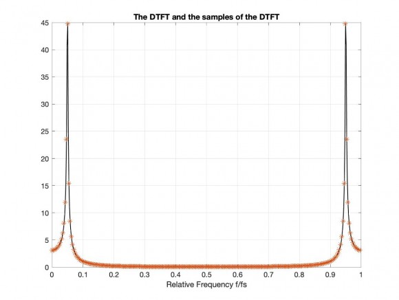
figure(2);   clf;

plot((0:nfft-1)/nfft, abs(X),'k-','LineWidth',1);

hold on;

plot((0:delta:nfft-1)/nfft, abs(Xr), '*');

title('The DTFT and the samples of the DTFT');

xlabel('Relative Frequency f/fs'); grid on;

figure(3);   clf;

subplot(211);  plot((0:nt-1)*Ts,x,'k-','LineWidth',1);

title('Original signal');   xlabel('Time in s');   grid on;

subplot(212);  plot((0:nfft-1)*Ts,real(xr),'k-','LineWidth',1); 

title('The reconstracted Signal from the subsampled DTFT');   

xlabel('Time in s');   grid on;    axis tight;

timealiasing_1.m

Hello,

Thank you very much for your reply. That is an interesting Matlab script.

However, (and please correct me if I am wrong here) but the code that you showed is taking the FFT of a time domain signal, under sampling it in the frequency domain, and then converting back to the time domain where the aliasing is visible.

However, I am starting off with my frequency response, H(w) and I would like to sample H(w) at evenly spaced frequencies to produce my DFT. Then I would like to take the IDFT to find my time domain signal. How can I effectively do this process without causing aliasing? 

Thank you for your time :D

Here is my Matlab Code to help explain what is going on (note, the bottom plots in windowed). The goal is that the top plot should be nearly identical to the bottom plot. After playing around with it for a while I've found that

b=ifft(h(1:30:end),30);

does produce somewhat good results. However, I don't think that I am properly doing this. it should be something like the below

b=ifft(h(1:2*pi/30:end),30);

plot:

code:

close all;
clear;
clc;

%list of frequency points to (normaled by pi)
f = [0 .1 .2 .3 .4 .5 .6 .7 .8 1];
%list of desired magnitude at the above points (low pass as an example)
a = [1 1 1 0 0 0 0 0 0 0];
taps=30;
n=taps-1;
b=firpm(n,f,a);%zeros of transfer function (i.e b0 b1*z^-1 ....)
[h,w2] = freqz(b,1,512); %plots the impulse response of the FIR and compares it to the ideal

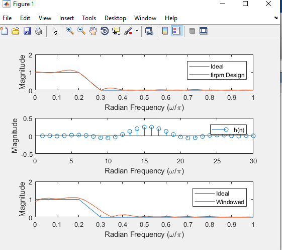
figure(1)
subplot(3,1,1)
plot(f,a,w2/pi,abs(h))
legend('Ideal','firpm Design')
xlabel 'Radian Frequency (\omega/\pi)', ylabel 'Magnitude'
subplot(3,1,2)
stem(b)
legend('h(n)')
xlabel 'Radian Frequency (\omega/\pi)', ylabel 'Magnitude'
subplot(3,1,3)
N = 22; %window Length (less than 30)
H = 0;
w=0:.1:pi;
b=ifft(h(1:30:end),30);%here, h is H(w), I think this is where I am messing up

for n=0:N-1 %windowing
    H = H + b(n+1)*exp(-1i*n.*w);
end
plot(f,a,w/pi,abs(H))
legend('Ideal','Windowed')
xlabel 'Radian Frequency (\omega/\pi)', ylabel 'Magnitude'

I think that your problem is the mismatch between your step through h in the ifft() and your actual frequency response - which (I think) is kinda what you said at the top.

You say that h should be h(1:2*pi/30:end), but that can't work because the indices are integers.  You want the steps to correspond with the sampled frequency, though.

h is from freqz() for which you requested 512 points.  512 doesn't divide evenly by 30, so you are calling your ifft() with a batch of h values that don't correspond with your intended/required frequencies - causing a shift in your mag response.

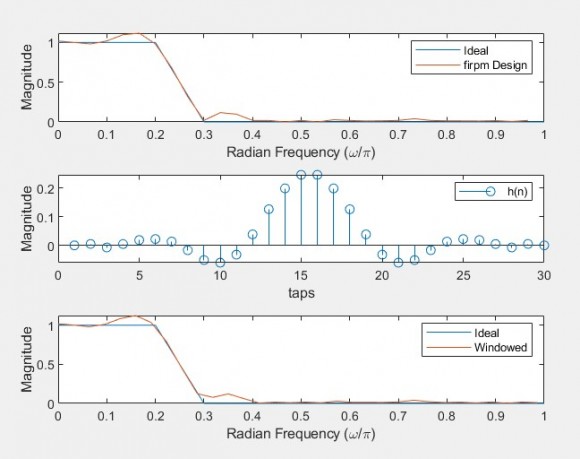
Without digging into it much, I changed your freqz() to 30 points to correct the misalignment, change the ifft line to: 

bb=ifft(h(1:2:30),30,'symmetric');

...and lengthened your window to the full length.  The correspondence between the top and bottom plots is now better.

Hello,

Thank you so much for your reply. That does make sense that my freqz and ifft should be using the same N. Your recommendations did give my the results that I initially expected. From this though, I have 2 more questions:

1) for the line of code, ifft(h(1:2:30),30,'symmetric'), why did you choose to step by 2 (i.e h(1:2:30) )? Also, why did you choose to add, 'symmetric' to the function?

2) For a different problem, suppose that I have a Matlab array of values, call it H_w that is my frequency response H(w). My goal is to get my FIR coefficients, h(n) from H(w). What information would I need in order to take ifft(H_w,...)?

Thanks again.

Hello AL,

Sorry for delay in getting back here.  The university semester is ending and I do not have much spare time with writing exams and all. 

The reason for the step was to account for the different form of freqz() and ifft().  freqz() is giving you a onesided response from 0 to pi and ifft is looking for a 0 to 2pi.  Alternatively, you could build the full input to ifft() by requesting a 15 length from freqz() and concatenating its forward and reverse as an input to ifft().  The 'symmetric' choice was more arbitrary on my part.  It helps to minimize rounding errors if they exist.

To your second question... you have what you need - the complex form of the frequency response.  You just need to construct the proper input to ifft() and go.   

That makes sense. Thank you for your help.

Just out of curiosity, what University do you teach at?

You are welcome.  I teach at Valparaiso University.  ...a small school southeast of Chicago.

Hello,

the following MATLAB-Script might help you:

%################################################

% Script sampled_mag_1.m, in which the impulse response of 

% a FIR Filter from the sampled magnitude is determined

clear;

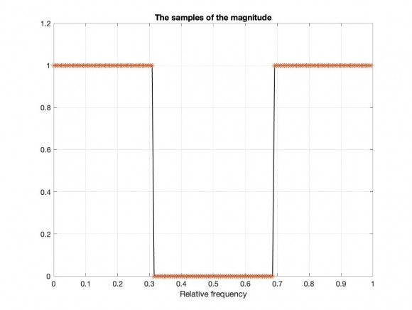
% ------- One period of the ideal sampled magnitude (zero phase)

Hi = [ones(1,50)  zeros(1,60) ones(1,49)];    nh = length(Hi);

figure(1);    clf;

plot((0:nh-1)/nh, abs(Hi),'k-','LineWidth',1);

hold on;

plot((0:nh-1)/nh, abs(Hi),'*');

hold off;

La = axis;    axis([La(1:2), La(3), 1.2]);

title('The samples of the magnitude');   grid on; 

xlabel('Relative frequency');

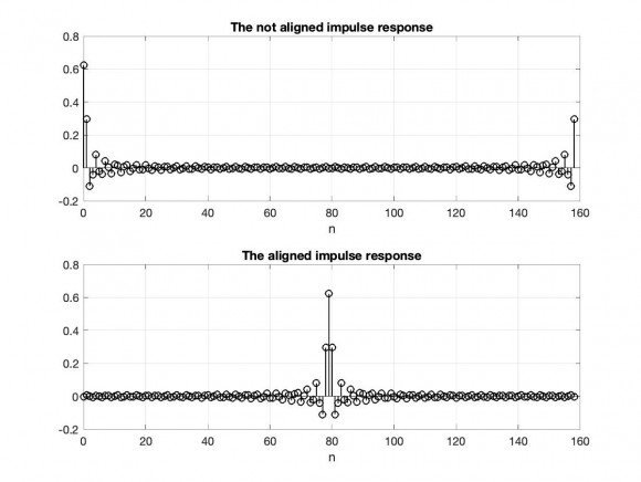
% ------- Impulse response

nfft = 256;               nfft >= nh;

hi = real(ifft(Hi));   % The imaginary are 0

figure(2);     clf;

subplot(211),  stem(0:nh-1, hi,'k-','LineWidth',1);

title('The not aligned impulse response');

xlabel('n');    grid on;

hia = fftshift(hi);      % aligning the impulse response

subplot(212),  stem(0:nh-1, hia,'k-','LineWidth',1);

title('The aligned impulse response');

xlabel('n');    grid on;

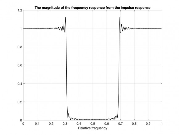
% ------- The magnitude from the hia impulse response

nfft = 256;               nfft >= nh;

Hia = fft(hia, nfft);

figure(3);     clf;

plot((0:nfft-1)/nfft, abs(Hia),'k-','LineWidth',1);

title(['The magnitude of the frequency responce from the',...

' impulse response']);

xlabel('Relative frequency');   grid on;

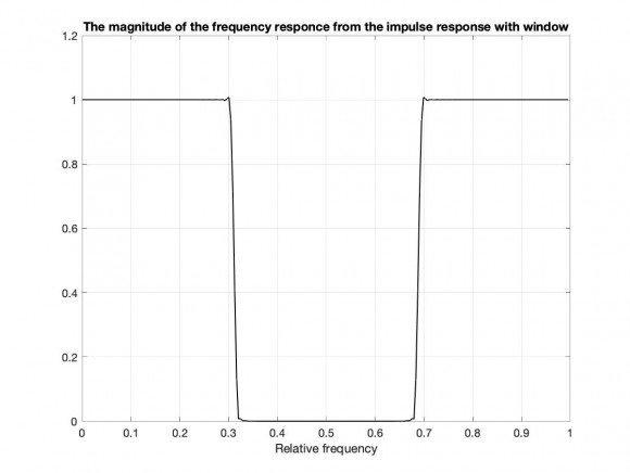
% ------- The magnitude from the impulse response with window

hiw = hia.*hann(nh)';

Hiw = fft(hiw, nfft);

figure(4);     clf;

plot((0:nfft-1)/nfft, abs(Hiw),'k-','LineWidth',1);

title(['The magnitude of the frequency responce from the',...

' impulse response with window']);

xlabel('Relative frequency');   grid on;

###########################################

sampled_mag_1.m

Late to the party, I know.  But I'm not understanding the X axis in the center plots in transient's and djmaguire's posts on April 24, 2020.  If h(n) is the impulse response, how can its units be Radian Frequency?  Shouldn't it be samples or time units?  Or did I miss something?  Thanks.  -Jim

Hi Jim,

You didn't miss anything.  That is a typo from the original MATLAB code posted by the OP.  All of the plot x-axes labels are set the same, inadvertently.  The center should be samples or coefficients or taps or something related.  I wasn't looking at the existing plot labels that closely.

If I get a chance, I'll update the figure that I posted.  The OP will have to change his original code and plot.  Thanks for noting!

Best,

Dan

Thanks, Dan.  Yeah, it didn't make sense to me.  Not that I'm a DSP expert, mind you.  Mostly my background is RF and microwave comms, but good to know DSP as well.  The discrete time domain is still quite mysterious to me!  -Jim

Hello Jim.

Ha ha. Don't worry. The discrete time domain is, every now and then, mysterious to us all.

is this what you want? reverse freqz output back to coeffs, then follow below:

f = [0 .1 .2 .3 .4 .5 .6 .7 .8 1];

a = [1 1 1 0 0 0 0 0 0 0];

b = fir2(29,f,a); %fir2 available to me

[h,w2] = freqz(b,1,30,'whole'); 

y = ifft(h);

plot(real(y)); hold;

plot(b,'r--');

Hi Kaz,

Thanks for your post. Your code does make sense.

I have found that most of my problems are orbiting my lack of understanding of  the Matlab functions freqz() and ifft(). Now that I have a better handle on how those work I think I am all set (see DJ Maguire's posts above).

Thanks again,

James